UFLDL Exercise:PCA and Whitening

1. result

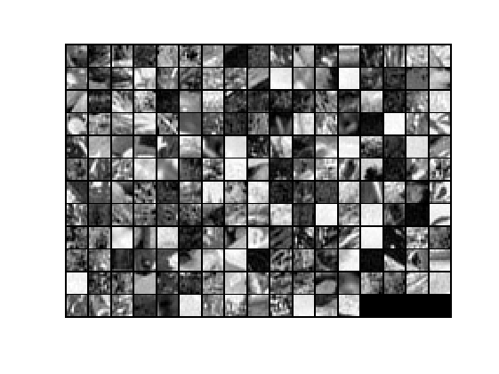
Raw images

Visualisation of Rot covariance matrix

PCA processed images(89/144 dimensions)

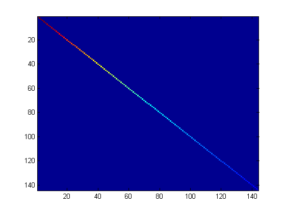
Visualisation of PCAWhite covariance matrix(epsilon = 0.1)

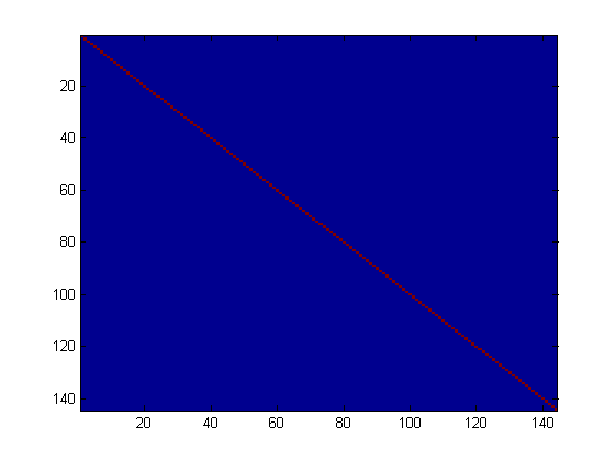
Visualisation of PCAWhite covariance matrix(epsilon = 0)

ZCA whitened images

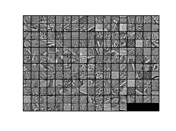
2. code

%%================================================================
%% Step 0a: Load data
%  Here we provide the code to load natural image data into x.
%  x will be a 144 * 10000 matrix, where the kth column x(:, k) corresponds to
%  the raw image data from the kth 12x12 image patch sampled.
%  You do not need to change the code below.

x = sampleIMAGESRAW();
figure('name','Raw images');
randsel = randi(size(x,2),200,1); % A random selection of samples for visualization
display_network(x(:,randsel));

%%================================================================
%% Step 0b: Zero-mean the data (by row)
%  You can make use of the mean and repmat/bsxfun functions.

% -------------------- YOUR CODE HERE -------------------- 
%x = bsxfun(@minus, x, mean(x, 1));
%%================================================================
%% Step 1a: Implement PCA to obtain xRot
%  Implement PCA to obtain xRot, the matrix in which the data is expressed
%  with respect to the eigenbasis of sigma, which is the matrix U.


% -------------------- YOUR CODE HERE -------------------- 
xRot = zeros(size(x)); % You need to compute this
sigma = x * x' / size(x, 2);
[u,s,v] = svd(sigma);
xRot = u' * x;

%%================================================================
%% Step 1b: Check your implementation of PCA
%  The covariance matrix for the data expressed with respect to the basis U
%  should be a diagonal matrix with non-zero entries only along the main
%  diagonal. We will verify this here.
%  Write code to compute the covariance matrix, covar. 
%  When visualised as an image, you should see a straight line across the
%  diagonal (non-zero entries) against a blue background (zero entries).

% -------------------- YOUR CODE HERE -------------------- 
covar = zeros(size(x, 1)); % You need to compute this
covar = xRot * xRot' /size(xRot, 2);
% Visualise the covariance matrix. You should see a line across the
% diagonal against a blue background.
figure('name','Visualisation of covariance matrix');
imagesc(covar);

%%================================================================
%% Step 2: Find k, the number of components to retain
%  Write code to determine k, the number of components to retain in order
%  to retain at least 99% of the variance.

% -------------------- YOUR CODE HERE -------------------- 
k = 0; % Set k accordingly
sums = 0;
for i=1:size(x,1)
    sums = sums + s(i, i);
    if sums >= 0.99 * sum(diag(s))
        k = i;
        break;
    end
end

%%================================================================
%% Step 3: Implement PCA with dimension reduction
%  Now that you have found k, you can reduce the dimension of the data by
%  discarding the remaining dimensions. In this way, you can represent the
%  data in k dimensions instead of the original 144, which will save you
%  computational time when running learning algorithms on the reduced
%  representation.
% 
%  Following the dimension reduction, invert the PCA transformation to produce 
%  the matrix xHat, the dimension-reduced data with respect to the original basis.
%  Visualise the data and compare it to the raw data. You will observe that
%  there is little loss due to throwing away the principal components that
%  correspond to dimensions with low variation.

% -------------------- YOUR CODE HERE -------------------- 
xHat = zeros(size(x));  % You need to compute this
tx = xRot;
tx(k+1:size(xRot,1), :) = zeros(size(xRot,1)-k, size(xRot,2));
xHat = u * tx;

% Visualise the data, and compare it to the raw data
% You should observe that the raw and processed data are of comparable quality.
% For comparison, you may wish to generate a PCA reduced image which
% retains only 90% of the variance.

figure('name',['PCA processed images ',sprintf('(%d / %d dimensions)', k, size(x, 1)),'']);
display_network(xHat(:,randsel));
figure('name','Raw images');
display_network(x(:,randsel));

%%================================================================
%% Step 4a: Implement PCA with whitening and regularisation
%  Implement PCA with whitening and regularisation to produce the matrix
%  xPCAWhite. 

epsilon = 0.1;
xPCAWhite = zeros(size(x));

% -------------------- YOUR CODE HERE -------------------- 
xPCAWhite = diag(1./sqrt(diag(s)+epsilon)) * xRot;
%%================================================================
%% Step 4b: Check your implementation of PCA whitening 
%  Check your implementation of PCA whitening with and without regularisation. 
%  PCA whitening without regularisation results a covariance matrix 
%  that is equal to the identity matrix. PCA whitening with regularisation
%  results in a covariance matrix with diagonal entries starting close to 
%  1 and gradually becoming smaller. We will verify these properties here.
%  Write code to compute the covariance matrix, covar. 
%
%  Without regularisation (set epsilon to 0 or close to 0), 
%  when visualised as an image, you should see a red line across the
%  diagonal (one entries) against a blue background (zero entries).
%  With regularisation, you should see a red line that slowly turns
%  blue across the diagonal, corresponding to the one entries slowly
%  becoming smaller.

% -------------------- YOUR CODE HERE -------------------- 
covar = xPCAWhite * xPCAWhite' / size(xPCAWhite, 2);%epsilon = 0 can get picture 5
% Visualise the covariance matrix. You should see a red line across the
% diagonal against a blue background.
figure('name','Visualisation of covariance matrix');
imagesc(covar);

%%================================================================
%% Step 5: Implement ZCA whitening
%  Now implement ZCA whitening to produce the matrix xZCAWhite. 
%  Visualise the data and compare it to the raw data. You should observe
%  that whitening results in, among other things, enhanced edges.

xZCAWhite = zeros(size(x));

% -------------------- YOUR CODE HERE -------------------- 
xZCAWhite = u * xPCAWhite;
% Visualise the data, and compare it to the raw data.
% You should observe that the whitened images have enhanced edges.
figure('name','ZCA whitened images');
display_network(xZCAWhite(:,randsel));
figure('name','Raw images');
display_network(x(:,randsel));