


如何将原始数据转换为合适处理时序预测问题的数据格式
如何准备数据并搭建LSTM来处理时序预测问题
如何利用模型预测
1.使用数据来源
该数据集来自kaggle竞赛的空气质量数据集 数据集来源
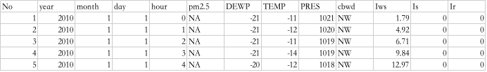
数据集包括日期、PM2.5浓度、露点、温度、风向、风速、累积小时雪量和累积小时雨量。原始数据中完整的特征如下:
| no | english | chinese |
|---|---|---|
| 1. | No | 行数 |
| 2. | year | 年 |
| 3. | month | 月 |
| 4. | day | 日 |
| 5. | hour | 小时 |
| 6. | pm2.5 | PM2.5浓度 |
| 7. | DEWP | 露点 |
| 8. | TEMP | 温度 |
| 9. | PRES | 大气压 |
| 10. | cbwd | 风向 |
| 11. | lws | 风速 |
| 12. | ls | 累积雪量 |
| 13. | lr | 累积雨量 |
- 我们可以利用此数据集搭建预测模型,利用前一个或几个小时的天气条件和污染数据预测下一个(当前)时刻的污染程度。
2.data processing
- first step:clear the data
第一步,我们必须清洗数据。以下是原始数据集的前几行。
- task1: 将日期整合为一个日期时间 方便做pandas的索引使用
- task2:需要快速显示前24H的pm2.5的NA值 删除 第一列的数据
- task3:在数据集中还有几个分散的NA值 现在可以用0值标记
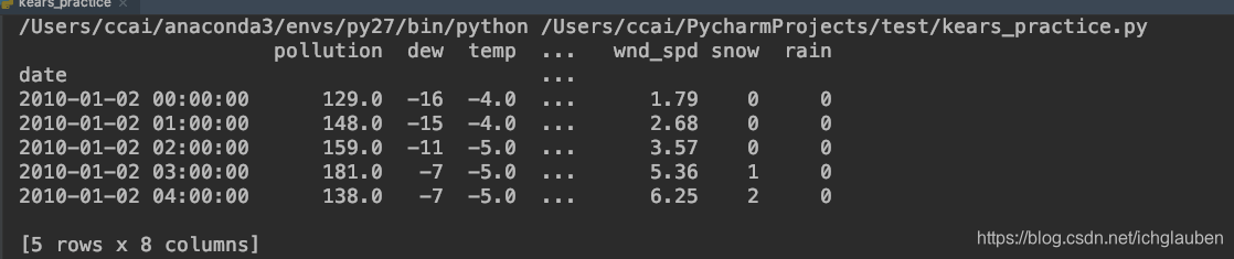
In summary:加载原始数据集,并将日期时间信息解析为Pandas Data Frame索引。“No”列被删除,然后为每列指定更清晰的名称。最后,将NA值替换为“0”值,并删除前24小时。
- 小demo:测试一下
inplace
>>> df = pd.DataFrame(np.arange(12).reshape(3,4),
...                   columns=['A', 'B', 'C', 'D'])
>>> df
   A  B   C   D
0  0  1   2   3
1  4  5   6   7
2  8  9  10  11
#结果替换了 + inplace=True
>>> df.drop('A',axis=1,inplace=True)
>>> df
   B   C   D
0  1   2   3
1  5   6   7
2  9  10  11


>>> df.insert(0,'A',[0,4,8])
>>> df
   A  a   b   c
A
0  0  1   2   3
1  4  5   6   7
2  8  9  10  11
>>> df.drop('A',axis=1)
#结果没有替换 只是copy
   a   b   c
A
0  1   2   3
1  5   6   7
2  9  10  11
>>> df
   A  a   b   c
A
0  0  1   2   3
1  4  5   6   7
2  8  9  10  11
# data processing
# first step :将日期时间 整合为一个日期时间 同时需要快速显示前24h的pm2.5
#的NA值 需要删除第一行no 还有分散的NA值 用0标记
# 转换时间为str
def parse(x):
    return datetime.strptime(x,'%Y %m %d %H')
# datetime.strptime()把一个时间字符串解析为时间元组
#time.strptime(string,[format])

#load data
dataset = read_csv('PRSA_data_2010.1.1-2014.12.31 2.csv',parse_dates=[['year','month','day','hour']],index_col=0,date_parser=parse)
# api read_csv
#index_col:使用作为行标签的列 0/false 不使用行标签行为
#date_parser:function 传入方法 用来转换一个string序列列成为datetime instances的array
#parse_dates:输入booth,list,dict(def:False) list of lists e.g. If [[1, 3]] -> combine columns 1 and 3 and parse as a single date column.
dataset.drop('No',axis=1,inplace=True)
#api pandas.DataFrame.drop
#DataFrame.drop(labels=None, axis=0, index=None, columns=None, level=None, inplace=False, errors='raise')
#inplace:If True, do operation inplace and return None.
#一般drop只是copy 如果要替换需要用inplace=True

# mn names
dataset.columns = ['pollution','dew','temp','press','wnd_dir','wnd_spd','snow','rain']
# index名称命名
dataset.index.name = 'date'

# mark all NA values with 0
dataset['pollution'].fillna(0,inplace=True)
#drop the first 24 hours 截掉从24-到以后的数据
dataset = dataset[24:]
# summary the first 5 rows test 一下
print (dataset.head(5))
# save file
dataset.to_csv('pollution.csv')
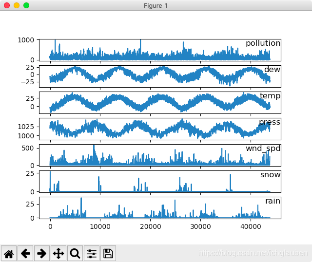
- 现在的数据格式已经更加适合处理,可以简单的对每列进行绘图。下面的代码加载了“pollution.csv”文件,并对除了类别型特性“风速”的每一列数据分别绘图。
visualization:
from pandas import read_csv
import matplotlib.pyplot as plt

# load_dataset
dataset = read_csv('pollution.csv',header=0,index_col=0)
#Explicitly pass header=0 to be able to replace existing names
values = dataset.values
#api: pd.values:output an array of values [[],[],[],...]

#specify columns to plot except the wind_speed column
groups = [0,1,2,3,5,6,7]
i = 1
#plot each column
plt.figure()
#create a image window
for group in groups:
    plt.subplot(len(groups),1,i)
    #plt.subplot:to create small images
    #divide the image window into len() rows,1 column,current position: i
    plt.plot(values[:,group])
    #values:rows(all),pick up the specific group
    plt.title(dataset.columns[group],y=1.0,loc='right')
    #fontdic: y=0.5 A dictionary controlling the appearance of the title text
    i += 1
plt.show()
3.多变量LSTM Model
3.1 make provision for the LSTM data
-
第一步是为LSTM准备污染数据集,涉及将数据集视为监督学习问题并对输入变量进行归一化处理。考虑到上一个时间段的污染测量和天气条件,我们将把监督学习问题作为预测当前时刻(t)的污染情况。根据过去24小时的天气情况和污染,预测下一个小时的污染,并给予下一个小时的“预期”天气条件。
-
可以使用
series_to_supervised()函数转换数据集 reference:将时间序列预测问题转换为py监督问题
series_to_supervised()函数
- 我们可以通过给定的输入和输出序列的长度,使用Pandas中的shift()函数自动创建新的时间序列问题的框架。
- 这将是一个有用的工具,因为它可以让我们使用机器学习算法探索不同框架的时间序列问题,来找到更好的模型。
- 在本节中,我们将定义一个名为series_to_supervised()的新Python函数,它采用单变量或多变量时间序列,并将其作为监督学习数据集
数据:序列,列表或二维的NumPy数组。 必需的参数。
n_in:作为输入的滞后步数(X)。 值可能介于[1..len(data)],可选参数。 默认为1。
n_out:作为输出的移动步数(y)。 值可以在[0..len(data)-1]之间, 可选参数。 默认为1。
dropnan:Boolean是否删除具有NaN值的行。 可选参数。 默认为True

return:
作为监督学习序列的Pandas DataFrame类型值。
新的数据集被构造为一个DataFrame,每一列都适当地以可变数量和时间步长命名。 这允许您从给定的单变量或多变量时间序列中设计各种不同的时间步长序列类型预测问题。
一旦DataFrame返回,您可以决定如何将返回的DataFrame的行分割为X和Y两部分,以便以任何您希望的方式监督学习。
这个函数是用默认参数定义的,所以如果你只用你的数据调用它,它将构造一个DataFrame,其中t-1为X,t为y。
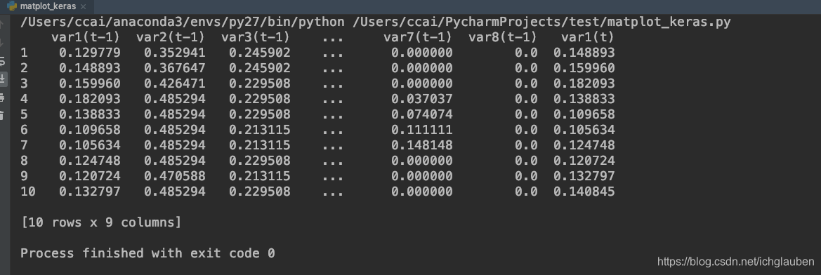
下面代码中首先加载“pollution.csv”文件,并利用sklearn的预处理模块对类别特征“风向”进行编码,当然也可以对该特征进行one-hot编码。 接着对所有的特征进行归一化处理,然后将数据集转化为有监督学习问题,同时将需要预测的当前时刻(t)的天气条件特征移除,完整代码如下:
from pandas import read_csv
import matplotlib.pyplot as plt
from  pandas import  DataFrame
from pandas import  concat
from sklearn.preprocessing import LabelEncoder, MinMaxScaler
def series_to_supersived(data,n_in=1,n_out=1,dropnan=True):
    """
    	Frame a time series as a supervised learning dataset.
    	Arguments:
    		data: Sequence of observations as a list or NumPy array.
    		n_in: Number of lag observations as input (X).
    		n_out: Number of observations as output (y).
    		dropnan: Boolean whether or not to drop rows with NaN values.
    	Returns:
    		Pandas DataFrame of series framed for supervised learning.
    """
    n_vars = 1 if type(data) is list else data.shape[1]
    df = DataFrame(data)
    cols,names = list(),list()
    #input sequence(t-n,...t-1)
    for i in range(n_in,0,-1):
        cols.append(df.shift(i))
        names += [('var%d(t-%d)' % (j+1,i)) for j in range(n_vars)]
    #forecast sequence (t,t+1,...t+n)
    for i in range(0,n_out):
        cols.append(df.shift(-i))
        if i == 0:
            names += [('var%d(t)' % (j+1)) for j in range(n_vars)]
        else:
            names += [('var%d(t+%d)' % (j+1,i)) for j in range(n_vars)]
    # put it all together
    agg = concat(cols,axis=1)
    agg.columns = names
    #drop rows with Nan values
    if dropnan:
        agg.dropna(inplace=True)
    return agg

#load data
dataset = read_csv('pollution.csv',header=0,index_col=0)
values = dataset.values
#integer encode direction
encoder = LabelEncoder()
values[:,4] = encoder.fit_transform(values[:,4])
#ensure all data is float
values = values.astype('float32')
#normalize feature
scaler =MinMaxScaler(feature_range=(0,1))
scaled = scaler.fit_transform(values)
# frame as supervised learning
reframed = series_to_supersived(scaled,1,1)
#drop columns we dont want to predict
reframed.drop(reframed.columns[[9,10,11,12,13,14,15]], axis=1, inplace=True)
print (reframed.head(10))
3.2build models
- 首先,我们需要将处理后的数据集划分为训练集和测试集。为了加速模型的训练,我们仅利用第一年数据进行训练,然后利用剩下的4年进行评估。
下面的代码将数据集进行划分,然后将训练集和测试集划分为输入和输出变量,最终将输入(X)改造为LSTM的输入格式,即[samples,timesteps,features]。
def train_test(reframed):
#split into train & test sets
values = reframed.values
n_train_hours = 365 * 24
train = values[:n_train_hours,:]
test = values[n_train_hours:,:]
#split into input and outputs
train_X,train_y = train[:, :-1] ,train[:,-1]
test_X , test_y = test[:,:-1] , test[:,-1]
# reshape input to be 3D [samples,timestep,features]
# shape[0]: rows [1] columns
train_X = train_X.reshape((train_X.shape[0],1,train_X.shape[1]))
test_X = test_X.reshape((test_X.shape[0],1,test_X.shape[1]))
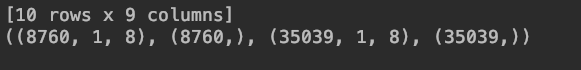
print(train_X.shape,train_y.shape,test_X.shape,test_y.shape)
return train_X,train_y,test_X,test_y
build model
- 现在可以搭建LSTM模型了。 LSTM模型中,隐藏层有50个神经元,输出层1个神经元(回归问题),输入变量是一个时间步(t-1)的特征,损失函数采用Mean Absolute Error(MAE),优化算法采用Adam,模型采用50个epochs并且每个batch的大小为72。
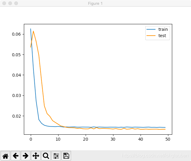
- 最后,在fit()函数中设置validation_data参数,记录训练集和测试集的损失,并在完成训练和测试后绘制损失图。
# design network
model = Sequential()
model.add(LSTM(50, input_shape=(train_X.shape[1], train_X.shape[2])))
model.add(Dense(1))
model.compile(loss='mae', optimizer='adam')
# fit network
history = model.fit(train_X, train_y, epochs=50, batch_size=72, validation_data=(test_X, test_y), verbose=2, shuffle=False)
# plot history
pyplot.plot(history.history['loss'], label='train')
pyplot.plot(history.history['val_loss'], label='test')
pyplot.legend()
pyplot.show()
3.3 model evaluation
接下里我们对模型效果进行评估。
值得注意的是:需要将预测结果和部分测试集数据组合然后进行比例反转(invert the scaling),同时也需要将测试集上的预期值也进行比例转换。
(We combine the forecast with the test dataset and invert the scaling. We also invert scaling on the test dataset with the expected pollution numbers.)
至于在这里为什么进行比例反转,是因为我们将原始数据进行了预处理(连同输出值y),此时的误差损失计算是在处理之后的数据上进行的,为了计算在原始比例上的误差需要将数据进行转化。同时笔者有个小Tips:就是反转时的矩阵大小一定要和原来的大小(shape)完全相同,否则就会报错。
通过以上处理之后,再结合RMSE(均方根误差)计算损失。
# make a prediction
yhat = model.predict(test_X)
test_X = test_X.reshape((test_X.shape[0], test_X.shape[2]))
# invert scaling for forecast
inv_yhat = concatenate((yhat, test_X[:, 1:]), axis=1)
inv_yhat = scaler.inverse_transform(inv_yhat)
inv_yhat = inv_yhat[:,0]
# invert scaling for actual
test_y = test_y.reshape((len(test_y), 1))
inv_y = concatenate((test_y, test_X[:, 1:]), axis=1)
inv_y = scaler.inverse_transform(inv_y)
inv_y = inv_y[:,0]
# calculate RMSE
rmse = sqrt(mean_squared_error(inv_y, inv_yhat))
print('Test RMSE: %.3f' % rmse
源代码
from pandas import read_csv
import matplotlib.pyplot as plt
from  pandas import  DataFrame
from pandas import  concat
# coding=UTF-8

import numpy as np
import  pandas as pd
from pandas import read_csv
from datetime import datetime
from numpy import  concatenate


import pandas as pd
from datetime import datetime
from matplotlib import pyplot
from sklearn.preprocessing import LabelEncoder,MinMaxScaler
from sklearn.metrics import mean_squared_error
from keras.models import Sequential
from keras.layers import Dense
from keras.layers import LSTM
from numpy import concatenate
from math import sqrt
from sklearn.preprocessing import LabelEncoder, MinMaxScaler
from keras.models import Model,load_model, model_from_json, Sequential
from keras.layers import Dense
from keras.layers import LSTM

# data processing
# first step :将日期时间 整合为一个日期时间 同时需要快速显示前24h的pm2.5
#的NA值 需要删除第一行no 还有分散的NA值 用0标记
# 转换时间为str
def parse(x):
        return datetime.strptime(x,'%Y %m %d %H')
# datetime.strptime()把一个时间字符串解析为时间元组
#time.strptime(string,[format])
def read_raw():
        #load data
        dataset = read_csv('PRSA_data_2010.1.1-2014.12.31 2.csv',parse_dates=[['year','month','day','hour']],index_col=0,date_parser=parse)
        # api read_csv
        #index_col:使用作为行标签的列 0/false 不使用行标签行为
        #date_parser:function 传入方法 用来转换一个string序列列成为datetime instances的array
        #parse_dates:输入booth,list,dict(def:False) list of lists e.g. If [[1, 3]] -> combine columns 1 and 3 and parse as a single date column.
        dataset.drop('No',axis=1,inplace=True)
        #api pandas.DataFrame.drop
        #DataFrame.drop(labels=None, axis=0, index=None, columns=None, level=None, inplace=False, errors='raise')
        #inplace:If True, do operation inplace and return None.
        #一般drop只是copy 如果要替换需要用inplace=True

        # mn names
        dataset.columns = ['pollution','dew','temp','press','wnd_dir','wnd_spd','snow','rain']
        # index名称命名
        dataset.index.name = 'date'

        # mark all NA values with 0
        dataset['pollution'].fillna(0,inplace=True)
        #drop the first 24 hours 截掉第一天的24h的数据
        dataset = dataset[24:]
        # summary the first 5 rows test 一下
        print (dataset.head(5))
        # save file
        dataset.to_csv('pollution.csv')

def draw_pollution():
    # load_dataset
    dataset = read_csv('pollution.csv',header=0,index_col=0)
    #Explicitly pass header=0 to be able to replace existing names
    values = dataset.values
    #api: pd.values:output an array of values [[],[],[],...]

    #specify columns to plot except the wind_speed column
    groups = [0,1,2,3,5,6,7]
    i = 1
    #plot each column
    plt.figure()
    #create a image window
    for group in groups:
        plt.subplot(len(groups),1,i)
        #plt.subplot:to create small images
        #divide the image window into len() rows,1 column,current position: i
        plt.plot(values[:,group])
        #values:rows(all),pick up the specific group
        plt.title(dataset.columns[group],y=1.0,loc='right')
        #fontdic: y=0.5 A dictionary controlling the appearance of the title text
        i += 1
    plt.show()


def series_to_supersived(data,n_in=1,n_out=1,dropnan=True):
    """
    	Frame a time series as a supervised learning dataset.
    	Arguments:
    		data: Sequence of observations as a list or NumPy array.
    		n_in: Number of lag observations as input (X).
    		n_out: Number of observations as output (y).
    		dropnan: Boolean whether or not to drop rows with NaN values.
    	Returns:
    		Pandas DataFrame of series framed for supervised learning.
    """
    n_vars = 1 if type(data) is list else data.shape[1]
    df = DataFrame(data)
    cols,names = list(),list()
    #input sequence(t-n,...t-1)
    for i in range(n_in,0,-1):
        cols.append(df.shift(i))
        names += [('var%d(t-%d)' % (j+1,i)) for j in range(n_vars)]
    #forecast sequence (t,t+1,...t+n)
    for i in range(0,n_out):
        cols.append(df.shift(-i))
        if i == 0:
            names += [('var%d(t)' % (j+1)) for j in range(n_vars)]
        else:
            names += [('var%d(t+%d)' % (j+1,i)) for j in range(n_vars)]
    # put it all together
    agg = concat(cols,axis=1)
    agg.columns = names
    #drop rows with Nan values
    if dropnan:
        agg.dropna(inplace=True)
    return agg

def cs_to_sl():
        #load data
        dataset = read_csv('pollution.csv',header=0,index_col=0)
        values = dataset.values
        #integer encode direction
        encoder = LabelEncoder()
        values[:,4] = encoder.fit_transform(values[:,4])
        #ensure all data is float
        values = values.astype('float32')
        #normalize feature
        scaler =MinMaxScaler(feature_range=(0,1))
        scaled = scaler.fit_transform(values)
        # frame as supervised learning
        reframed = series_to_supersived(scaled,1,1)
        #drop columns we dont want to predict
        reframed.drop(reframed.columns[[9,10,11,12,13,14,15]], axis=1, inplace=True)
        print (reframed.head(10))
        return  reframed,scaler

def train_test(reframed):
    #split into train & test sets
    values = reframed.values
    n_train_hours = 365 * 24
    train = values[:n_train_hours,:]
    test = values[n_train_hours:,:]
    #split into input and outputs
    train_X,train_y = train[:, :-1] ,train[:,-1]
    test_X , test_y = test[:,:-1] , test[:,-1]
    # reshape input to be 3D [samples,timestep,features]
    # shape[0]: rows [1] columns
    train_X = train_X.reshape((train_X.shape[0],1,train_X.shape[1]))
    test_X =  test_X.reshape((test_X.shape[0],1,test_X.shape[1]))
    print(train_X.shape,train_y.shape,test_X.shape,test_y.shape)
    return train_X,train_y,test_X,test_y

def fit_network(train_X,train_y,test_x,test_y,scaler):
    model = Sequential()
    model.add(LSTM(50,input_shape=(train_X.shape[1],train_X.shape[2])))
    model.add(Dense(1))
    model.compile(loss='mae',optimizer='adam')
    #fit network
    history = model.fit(train_X,train_y,epochs=50,batch_size=72,validation_data=(test_x,test_y),verbose=2,shuffle=False)
    # plot history
    plt.plot(history.history['loss'],label='train')
    plt.plot(history.history['val_loss'],label='test')
    plt.legend()
    plt.show()
    # make a prediction
    yhat = model.predict(test_x)
    test_x = test_x.reshape((test_x.shape[0],test_x.shape[2]))
    #invert scaling for forecast
    inv_yhat = concatenate((yhat,test_x[:,1:]),axis=1)
    inv_yhat = scaler.inverse_transform(inv_yhat)
    inv_yhat = inv_yhat[:,0]
    #invert scaling for actual
    inv_y = scaler.inverse_transform(test_x)
    inv_y = inv_y[:,0]
    #calculate RMSE
    rmse = sqrt(mean_squared_error(inv_y,inv_yhat))
    print('test RMSE: {%.3f}'.format(rmse) )


if __name__ == '__main__':
    draw_pollution()
    reframed,scaler = cs_to_sl()
    train_test(reframed)
    train_X,train_y,test_X,test_y = train_test(reframed)
    fit_network(train_X,train_y,test_X,test_y,scaler)


 5809
5809


 被折叠的 条评论
为什么被折叠?
被折叠的 条评论
为什么被折叠?
 到【灌水乐园】发言


