


 本文介绍了一种用于时间序列分析的神经网络模型,该模型能够将序列分解为周期性和非周期性成分,通过学习数据自动调整频谱。文章提供了详细的模型结构、训练过程和预测效果,并对比了与prophet模型的不同之处。
论文及代码
原始论文:
代码:https://github.com/trokas/neural_decomposition
模型
将时间序列分解成周期项和非周期项 g ( t ) g(t) g(t):
x ( t ) = ∑ k = 1 N ( a k ⋅ sin ( w k t + ϕ k ) ) + g ( t ) . x(t) = \sum _{k = 1}^{N}{( a_{k} \cdot \sin ( w_{k} t + \phi _{k} )) } + g(t). x(t)=k=1∑N(ak⋅sin(wkt+ϕk))+g(t).
其中 a k , w k , ϕ k a_k, w_k, \phi_k ak,wk,ϕk 和 g ( t ) g(t) g(t) 都需要从数据中学习。
网络结构为:
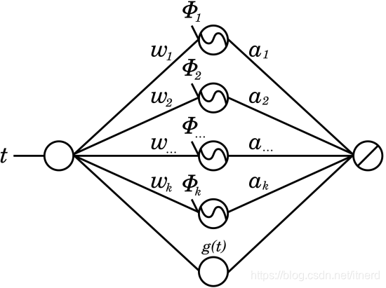
其中
g
(
t
)
g(t)
g(t) 可以理解为序列的趋势项,主要考虑线性趋势
w
t
+
b
wt+b
wt+b,sigmoid函数,softplus函数等等。
这个模型很容易让人想到 prophet 模型,甚至是 prophet 的简化版,因为 prophet 好歹考虑的是分段线性趋势,还有节假日带来的影响。不过这个模型的优势在于可以通过数据来调节频谱,而 prophet 是从预先给定的频谱中筛选频谱。
代码
参见上述 github 地址,用 keras 实现起来太简单啦,,,
model
%matplotlib inline
import matplotlib.pyplot as plt
import seaborn
import numpy as np
import pandas as pd
from keras.models import Input, Model, Sequential
from keras.layers.core import Dense
from keras.layers.merge import Concatenate
from keras.layers import LSTM, Activation
from keras import regularizers
from scipy.interpolate import interp1d
from fbprophet import Prophet

plt.rcParams['figure.figsize'] = [12.0, 8.0]


def create_model(n, units=10, noise=0.001):
    """
    Constructs neural decomposition model and returns it
    """
    data = Input(shape=(1,), name='time')
    # sin will not work on TensorFlow backend, use Theano instead
    sinusoid = Dense(n, activation=np.sin, name='sin')(data)
    linear = Dense(units, activation='linear', name='linear')(data)
    softplus = Dense(units, activation='softplus', name='softplus')(data)
    sigmoid = Dense(units, activation='sigmoid', name='sigmoid')(data)
    combined = Concatenate(name='combined')([sinusoid, linear, softplus, sigmoid])
    out = Dense(1, kernel_regularizer=regularizers.l1(0.01), name='output')(combined)

    model = Model(inputs=[data], outputs=[out])
    model.compile(loss="mse", optimizer="adam")

    model.weights[0].set_value((2*np.pi*np.floor(np.arange(n)/2))[np.newaxis,:].astype('float32'))
    model.weights[1].set_value((np.pi/2+np.arange(n)%2*np.pi/2).astype('float32'))
    model.weights[2].set_value((np.ones(shape=(1,units)) + np.random.normal(size=(1,units))*noise).astype('float32'))
    model.weights[3].set_value((np.random.normal(size=(units))*noise).astype('float32'))
    model.weights[4].set_value((np.random.normal(size=(1,units))*noise).astype('float32'))
    model.weights[5].set_value((np.random.normal(size=(units))*noise).astype('float32'))
    model.weights[6].set_value((np.random.normal(size=(1,units))*noise).astype('float32'))
    model.weights[7].set_value((np.random.normal(size=(units))*noise).astype('float32'))
    model.weights[8].set_value((np.random.normal(size=(n+3*units,1))*noise).astype('float32'))
    model.weights[9].set_value((np.random.normal(size=(1))*noise).astype('float32'))

    return model
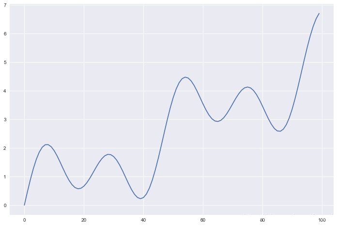
测试序列
t = np.linspace(0, 1, 100)
X = np.sin(4.25*np.pi*t) + np.sin(8.5*np.pi*t) + 5*t
plt.plot(X)
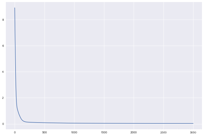
训练
%%time
model = create_model(len(X))
hist = model.fit(t, X, epochs=3000, verbose=0)
plt.plot(hist.history['loss'])
Wall time: 15.8 s
预测
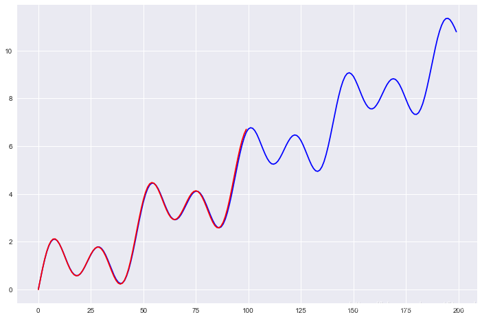
prediction = model.predict(np.linspace(0, 2, 200)).flatten()

plt.plot(prediction, color='blue')
plt.plot(X, color='red')
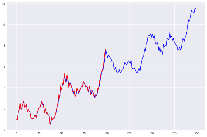
加点噪声
t = np.linspace(0, 1, 100)
X = np.sin(4.25*np.pi*t) + np.sin(8.5*np.pi*t) + 5*t + np.random.uniform(size=100)
model = create_model(len(X))
hist = model.fit(t, X, epochs=3000, verbose=0)
prediction = model.predict(np.linspace(0, 2, 200)).flatten()
plt.plot(prediction, color='blue')
plt.plot(X, color='red')
pytorch 实现
class ND(nn.Module):
    def __init__(self, n, units=10, noise=0.001):
        super(ND, self).__init__()
        self.wave = nn.Linear(1, n)
        self.unit_linear = nn.Linear(1, units)
        self.unit_softplus = nn.Linear(1, units)
        self.unit_sigmoid = nn.Linear(1, units)
        self.fc = nn.Linear(n + 3*units, 1)
        # Initialize weights
        params = dict(self.named_parameters())
        params['wave.weight'].data = torch.from_numpy((2*np.pi*np.floor(np.arange(n)/2))[:,np.newaxis]).float()
        params['wave.bias'].data = torch.from_numpy(np.pi/2+np.arange(n)%2*np.pi/2).float()
        params['unit_linear.weight'].data = torch.from_numpy(np.ones(shape=(units,1)) + np.random.normal(size=(units,1))*noise).float()
        params['unit_linear.bias'].data = torch.from_numpy(np.random.normal(size=(units))*noise).float()
        params['unit_softplus.weight'].data = torch.from_numpy(np.random.normal(size=(units,1))*noise).float()
        params['unit_softplus.bias'].data = torch.from_numpy(np.random.normal(size=(units))*noise).float()
        params['unit_sigmoid.weight'].data = torch.from_numpy(np.random.normal(size=(units,1))*noise).float()
        params['unit_sigmoid.bias'].data = torch.from_numpy(np.random.normal(size=(units))*noise).float()
        params['fc.weight'].data = torch.from_numpy(np.random.normal(size=(1,n+3*units))*noise).float()
        params['fc.bias'].data = torch.from_numpy(np.random.normal(size=(1))*noise).float()

    def forward(self, x):
        sinusoid = torch.sin(self.wave(x))
        linear = self.unit_linear(x)
        softplus = nn.Softplus()(self.unit_softplus(x))
        sigmoid = nn.Sigmoid()(self.unit_sigmoid(x))
        combined = torch.cat([sinusoid, linear, softplus, sigmoid], dim=1)
        out = self.fc(combined)
        return out

# x = np.linspace(0, 1.5, 150)
# x = np.sin(4.25*np.pi*x)+np.sin(8.5*np.pi*x)+5*x
x = np.linspace(0,1,100)[:, np.newaxis]
X = Variable(torch.from_numpy(x).float())
y = np.sin(np.linspace(0,20,100))[:, np.newaxis]
Y = Variable(torch.from_numpy(y).float())

nd = ND(x.shape[0])
print(nd)

# Loss and Optimizer
criterion = nn.MSELoss()
optimizer = torch.optim.Adam(nd.parameters())

# Train the Model
for epoch in range(2000):
    # Forward + Backward + Optimize
    optimizer.zero_grad()  # zero the gradient buffer
    outputs = nd.forward(X)
    loss = criterion(outputs, Y)

    # Add L1 to loss
    loss += 0.01*torch.sum(torch.abs(dict(nd.named_parameters())['fc.weight']))

    loss.backward()
    optimizer.step()

    if epoch % 100 == 0:
        print ('Epoch {0}, Loss: {1:.4f}'.format(epoch, loss.data[0]))


 391
391

 被折叠的 条评论
为什么被折叠?
被折叠的 条评论
为什么被折叠?
 到【灌水乐园】发言


