16数据处理

最新推荐文章于 2024-09-07 21:01:55 发布

sorry_maker

最新推荐文章于 2024-09-07 21:01:55 发布

阅读量359

点赞数

文章标签：人工智能数据处理 plotly pandas mongodb

本文链接：https://blog.csdn.net/jaken_xie/article/details/133465201

版权

plotly

设置x/y轴名称

yaxis_title=‘金额(元)’,xaxis_title=‘日期’

fig = px.line(df_grouped, x="Order_time", y="Money", title='日销图')
fig.update_layout(yaxis_title='金额(元)',xaxis_title='日期', xaxis_tickformat='%Y-%m-%d',yaxis_tickformat = '0.2f')
fig.show()

设置x/y轴范围

fig.update_layout(yaxis_title='loss',xaxis_title='epochs',yaxis_tickformat = '0.3f',
                  #全闭区间0-61
                  xaxis_range=[0,61]
                 )

调整日期格式

xaxis_tickformat='%Y-%m-%d

# 画图展示每日销量
fig = px.line(df_grouped, x="Order_time", y="Money", title='日销图')
fig.update_layout(yaxis_title='金额(元)',xaxis_title='日期', xaxis_tickformat='%Y-%m-%d',yaxis_tickformat = '0.2f')
fig.show()

设置数值保留小数

yaxis_tickformat = ‘0.2f’

# 画图展示每日销量
fig = px.line(df_grouped, x="Order_time", y="Money", title='日销图')
fig.update_layout(yaxis_title='金额(元)',xaxis_title='日期', xaxis_tickformat='%Y-%m-%d',yaxis_tickformat = '0.2f')
fig.show()

基础折线图

import plotly.express as px
# 画图展示每日销量
fig = px.line(df_final, x="Order_time", y="Money", title='日销图',hover_data=['count'])
fig.update_layout(yaxis_title='金额(元)',xaxis_title='日期', xaxis_tickformat='%Y-%m-%d',yaxis_tickformat = '0.2f')
fig.show()

去除网格

fig = go.Figure()
fig.update_layout(yaxis_title='loss',xaxis_title='epochs',yaxis_tickformat = '0.2f',xaxis_showgrid=False, yaxis_showgrid=False)

设置背景颜色

fig.update_layout(yaxis_title='loss',xaxis_title='epochs',yaxis_tickformat = '0.2f',xaxis_showgrid=False, yaxis_showgrid=False,paper_bgcolor='white',plot_bgcolor='rgb(243, 243, 243)')

一图多表

https://plotly.com/python/reference/scatter/

示例1

import plotly.graph_objects as go
fig = go.Figure()
fig.update_layout(yaxis_title='金额(元)',xaxis_title='日期', xaxis_tickformat='%Y-%m-%d',yaxis_tickformat = '0.2f')

fig.add_trace(go.Scatter(
    x=df_final_no_index['Order_time'],
    y=df_final_no_index['Money'],
    name = 'Real Price',
    # 设定图像的形式
    mode = 'lines',
    # 在marker中设置图像的颜色
#    marker = dict(
#         color = 'skyblue'，
#		  size =5,
#		  symbol = 'circle/square/x'
#     )
))
fig.add_trace(go.Scatter(
    x=df_final_no_index['Order_time'][-(test_split-30):],
    y=pred,
    name = 'Predicted Price',
    mode = 'lines'
))

fig.show()

示例2：

import plotly.graph_objects as go
fig = go.Figure()
fig.update_layout(yaxis_title='充值分数',xaxis_title='消费分数',yaxis_tickformat = '0.2f',title = '分类结果')

fig.add_trace(go.Scatter(
    x=total_data['consume_score'],
    y=total_data['recharge_score'],
    name = '用户分数',
    # 设定图像的形式
    mode = 'markers',
    marker = dict(
        color = total_data['prediction'],
        colorscale = 'Viridis'
    )
))
fig.add_trace(go.Scatter(
    x=centers['x'],
    y=centers['y'],
    name = '质心',
    mode = 'markers',
    marker = dict(
        size = 10,
        symbol = 'x'
    )
))

fig.show()

显示额外数据

hover_data

fig = px.line(df_final, x="Order_time", y="Money", title='日销图',hover_data=['count'])

pandas

索引

删除索引

df_final.reset_index(drop=False,inplace=True)

添加索引

df_final.set_index('Order_time',inplace=True)

分组及聚合操作

求和

# 按照日期分组并求和，会对能够计算的列进行求和  numeric_only防止警告
df_grouped_sum = df_clear.groupby(by=df_clear['Order_time'].dt.date).sum(numeric_only = True)

计数

# 按照日期分组并计数 会对所有列进行计数
df_grouped_count = df_clear.groupby(by=df_clear['Order_time'].dt.date).count()

ndarray转dataframe

array_1 = np.array([1, 2, 3, 4])
df_1 = pd.DataFrame(array_1, columns=["Column 1"])

concat根据索引合并

import numpy as np
import pandas as pd
# Create two ndarrays
array_1 = np.array([1, 2, 3, 4])
array_2 = np.array([5, 6, 7, 8])

# Convert ndarrays to DataFrames
df_1 = pd.DataFrame(array_1, columns=["Column 1"])
df_2 = pd.DataFrame(array_2, columns=["Column 2"])

# Concatenate DataFrames along columns (axis=1)
df_merged = pd.concat([df_1, df_2], axis=1)

print(df_merged)

修改列类型

older['Order_time'] = older['Order_time'].astype('str')

按列赋值

# 其中pred是ndarray类型也可以 df类型就指定列即可
df_test_predict['Money'] = pred

merge根据字段合并

In [33]: left = pd.DataFrame(
   ....:     {
   ....:         "key": ["K0", "K1", "K2", "K3"],
   ....:         "A": ["A0", "A1", "A2", "A3"],
   ....:         "B": ["B0", "B1", "B2", "B3"],
   ....:     }
   ....: )
   ....: 

In [34]: right = pd.DataFrame(
   ....:     {
   ....:         "key": ["K0", "K1", "K2", "K3"],
   ....:         "C": ["C0", "C1", "C2", "C3"],
   ....:         "D": ["D0", "D1", "D2", "D3"],
   ....:     }
   ....: )
   ....: 

In [35]: result = pd.merge(left, right, on="key")

读取文件

excel

df=pd.read_excel("data/Data003_SelfOperate.xlsx",parse_dates=["Order_time"])

查看数据范围

df.describe().loc[['min', 'max']]

去除时分秒

df["Order_time"] = df["Order_time"].dt.date

过滤数据

# 过滤金额范围
df = df[(df['Money']>=5)&(df['Money']<=10000)]
# 过滤时间段为[2020-1-1:]
df['Order_time'] = pd.to_datetime(df['Order_time'])
df = df[(df['Order_time'] >= pd.Timestamp('2020-01-01'))]

选择多列

df_clear = df[['Order_time','Money']]

插入新列

df.insert(loc=2, column='c', value=3)  # 在最后一列后，插入值全为3的c列

保留小数

df_merged['predicted_price'] = df_merged['predicted_price'].apply(lambda x: round(x, 2))

生成时间序列

pd_day = pd.date_range('20220708',periods=30,freq='D')

eg:

需求：在已有日期df_for_predict后加入新增的时间序列

# 创建空的数组
# empty = np.zeros((future_span,1))
# ndarray 转 pd
# future = pd.DataFrame(empty,columns = ['Money'])
# 生成时间序列
pd_day = pd.date_range('20220708',periods=future_span,freq='D')
# ndarray 转 pd
older = pd.DataFrame(pd_day,columns=['Order_time'])
# 时间类型转换成字符串
older['Order_time'] = older['Order_time'].astype('str')
# older.set_index('Order_time',inplace=True)
# 插入money列
older.insert(loc=1, column='Money', value=0)
# 按行连接两个表
df_for_predict = pd.concat([df_for_predict,older])
df_for_predict.set_index('Order_time',inplace=True)
df_for_predict.tail(20)

machine learning

激活函数 activation

作用

一个没有激活函数的神经网络将只不过是一个线性回归模型（Linear regression Model）罢了，它功率有限，并且大多数情况下执行得并不好。

将模型中一个节点的输入信号转换成一个输出信号,这使得模型可以学习和模拟其他复杂类型的数据。

比如逻辑回归中 $z = w x + b$

而激活函数的输入为z : $function=\frac{1}{1+e^{-z}}$

如何选择

在深度学习的隐藏层中，一般使用relu
在输出层，取决于标签值y
1. y=0/1 ——sigmoid
2. y可正可负——linear
3. y$>=$0——relu

loss函数和cost函数

loss:用来计算预测值与真实值之间的差异，是单个样本的值

比如逻辑回归中使用的交叉熵函数：

以及非逻辑回归的均方差函数：

cost:整个训练集上loss的平均值

模型的最终目的就是尽可能使cost函数最小化

loss值和val_loss值

loss和val loss 的区别：
loss：训练集整体的损失值。
val loss：验证集（测试集）整体的损失值。
loss和val loss，两者之间的关系：
当loss下降，val_loss下降：训练正常，最好情况。

当loss下降，val_loss稳定：网络过拟合化。这时候可以添加Dropout和Max pooling。
当loss稳定，val_loss下降：说明数据集有严重问题，可以查看标签文件是否有注释错误，或者是数据集质量太差。建议重新选择。
当loss稳定，val_loss稳定：学习过程遇到瓶颈，需要减小学习率（自适应网络效果不大）或batch数量。
当loss上升，val_loss上升：网络结构设计问题，训练超参数设置不当，数据集需要清洗等问题，最差情况

梯度下降

梯度下降法(alpha 为学习率):

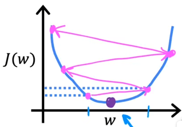
学习率

影响的是梯度下降的过程

过小：导致梯度下降过程缓慢

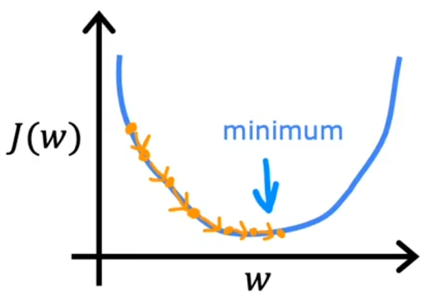
过大：可能永远达不到梯度的最小值

过拟合

解决方法

收集更多数据
不要使用太多特征
正则化

正则化

核心：尽可能地减小w(权重)，与直接删除某些特征值的做法相比，他更加温和

原理

目的是最小化代价函数J(w,b)

$\lambda=0$ :相当于没有正则化
$\lambda过大$ :要使得J尽可能小，那么w就尽可能小，因为他前面的系数 $\lambda$ 很大，导致w近似为0，出现欠拟合

所以 $\lambda$ 需要有合理的取值范围，通常为[1,10]

tensorflow

一般步骤

以逻辑回归为例，使用tf构造神经网络的步骤和机器学习中的步骤一样

构造模型
选取loss函数
评估

举例

定义模型

loss and cost

模型构造及loss观测

例：

model = Sequential()
model.add(LSTM(50, return_sequences=True,input_shape = (span,1)))
# model.add(LSTM(50))
model.add(Dropout(0.2))
model.add(Dense(1))
model.compile(loss = "mse",optimizer= "adam")
train_history =model.fit(trainX, trainY, epochs= 100, batch_size=50, validation_data=(testX, testY), verbose=1, shuffle=False)

# 画图
plt.figure()
plt.plot(train_history.history["loss"], label = "loss")
plt.plot(train_history.history["val_loss"], label = "val_loss")
plt.legend()
plt.show()

查看模型详情

model.summary()

sklearn

标准化处理

from sklearn.preprocessing import StandardScaler
# 标准化处理
scaler = StandardScaler()
df_for_training_scaled=scaler.fit_transform(df_for_training)

# 反标准化
scaler.inverse_transform(df_for_training)

归一化处理MinMaxScaler

from sklearn.preprocessing import MinMaxScaler
scaler = MinMaxScaler(feature_range=(0,1))
df_for_training_scaled=scaler.fit_transform(df_for_training)
df_for_testing_scaled=scaler.transform(df_for_testing)
df_for_training_scaled

两个特征值结果为：

GridSearchCV

参考博客

强烈推荐视频

例子

from tensorflow.keras.models import Sequential
from tensorflow.keras.layers import LSTM
from tensorflow.keras.layers import Dense, Dropout
from keras.wrappers.scikit_learn import KerasRegressor
from sklearn.model_selection import GridSearchCV
def build_model(optimizer):
    grid_model = Sequential()
    # 层数过少导致的问题就是预测的曲线会比较平滑
    grid_model.add(LSTM(60,return_sequences=True,input_shape=(span,1)))
    grid_model.add(LSTM(60))
    # grid_model.add(Dense(64,activation="relu"))
    # Dropout设置防止过拟合的参数,相当于正则化参数
    grid_model.add(Dropout(0.2))
    grid_model.add(Dense(1))
    # 用均方差(mse)作为loss函数
    grid_model.compile(loss = 'mse',optimizer = optimizer)
    return grid_model
# verbose=1设置打印的等级
grid_model = KerasRegressor(build_fn=build_model,verbose=1,validation_data=(testX,testY))
parameters = {'batch_size' : [5],
              # epochs为迭代次数
              'epochs' : [20],
              'optimizer' : ['adam'] }

grid_search  = GridSearchCV(estimator = grid_model,
                            param_grid = parameters,
                            # cv默认值是5折交叉验证
                           )

训练集样本数量是675
$每一轮的训练次数=108=\frac{675\times(\frac{cv-1=4}{cv=5})}{batch\_size=5}$

CV交叉验证参数

会将训练集分成CV份,其中 $\frac{CV-1}{CV}$ 份用来训练， $\frac{1}{CV}$ 用来验证(注意不是测试！！！)

eg:10折交叉验证

batch_size

会将CV之后的训练集在进行划分，每一份batch_size个

分数

print('Best: {} using {}'.format(grid_search.best_score_, grid_search.best_params_))

最终的分数是在CV交叉验证时针对验证集的拟合情况

所以GridCV中分数高，只代表它在交叉验证环节的分数高，针对的是验证集，但是如果将模型应用到测试集上时，结果并不一定是最好的

batch_size和epoch

一般来说，在合理的范围之内，越大的 batch size 使下降方向越准确，震荡越小

batch取太大会陷入局部最小值，

batch取太小loss会抖动厉害，因为过度关注了每一个数据（包括噪音），所以容易导致过拟合而不是欠拟合

batch_size：一次训练所选取的样本数; batch_size的大小影响内存的使用情况，同时也影响模型的优化程度和速度。

mongoDB

python + mongoDB

import json
# 连接MongoDB数据库
from pymongo import MongoClient
#连接Mongodb数据库
conn = MongoClient('192.168.10.1',27017)

def df2bson(df):
    """DataFrame类型转化为Bson类型"""
    data = json.loads(df.T.to_json()).values()
    return data

# df_data为要存储的数据  table为数据库中表的名称
def saveMongo(df_data,table):
    # userdata为数据库名称
    db = conn["userdata"]
    table = db[table]
    bson_data = df2bson(df_data)
    result = table.insert_many(bson_data)
# 将数据保存到mongodb中
saveMongo(raise_df,"user_raise")

时间戳转日期

https://blog.csdn.net/qq_45366447/article/details/128617142

db.daily_consume.aggregate([
    {
        $project: {
            "Order_time_formatted": {
                $dateToString: {
                    format: '%Y-%m-%d',
                    date: {
                        $add: [
                            ISODate('1970-01-01T00:00:00.000Z'),
                            '$Order_time',
                            28800000
                        ]
                    }
                }
            },
            "_id": "$_id"
        }
    }
]).forEach(function(doc) {
  db.daily_consume.update({
    "_id": doc._id
  }, {
    "$set": {
      "Order_time_formatted": doc.Order_time_formatted
    }
  });
});

在终端中输入上述命令，可以看到已经成功转变过来

regate([
{
$project: {
“Order_time_formatted”: {
$dateToString: {
format: ‘%Y-%m-%d’,
date: {
$a dd : [I SO D a t e (^{'} 1970 - 01 - 01 T 00 : 00 : 00.000 Z^{'}),^{'}$ Order_time’,
28800000
]
}
}
},
“_id”: “ $KaTeX parse error: Expected 'EOF', got '}' at position 14: _id" }̲ } ]).forEa\dots$ set”: {
“Order_time_formatted”: doc.Order_time_formatted
}
});
});


在终端中输入上述命令，可以看到已经成功转变过来

[外链图片转存中...(img-mUQrzypv-1696143131169)]

sorry_maker

关注

0
点赞
踩
0

收藏

觉得还不错? 一键收藏
0
评论
16数据处理

yaxis_title=‘金额(元)’,xaxis_title=‘日期’
复制链接

扫一扫