深度学习中的一些常见的激活函数集合（含公式与导数的推导）sigmoid, relu, leaky relu, elu， numpy实现

%matplotlib inline
%config InlineBackend.figure_format = "png"
import matplotlib.pyplot as plt
import numpy as np

plt.rcParams['figure.figsize'] = (8, 5)
plt.rcParams['figure.dpi'] = 150
plt.rcParams['font.sans-serif'] = ['Simhei']  #替代字体
plt.rcParams['axes.unicode_minus'] = False  #解决坐标轴负数的铅显示问题

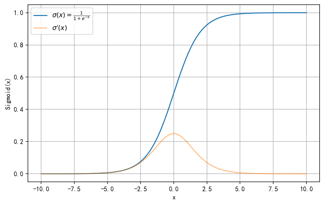
Sigmoid(x)

$$\text{sigmoid}(x)=\sigma (x)=\frac{1}{1+e^{-x}}$$

$\begin{array}{rl}{\sigma }^{\prime }(x)=& [(1+e^{-x}{)}^{-1}{]}^{\prime }\\ =& (-1)(1+e^{-x}{)}^{-2}(-1)e^{-x}\\ =& (1+e^{-x}{)}^{-2}{e}^{-x}\\ =& \frac{e^{-x}}{(1+e^{-x}{)}^2}\\ =& \frac{1+e^{-x}-1}{(1+e^{-x}{)}^2}\\ =& \frac{1+e^{-x}}{(1+e^{-x}{)}^2}-\frac{1}{(1+e^{-x}{)}^2}\\ =& \frac{1}{(1+e^{-x})}(1-\frac{1}{(1+e^{-x})})\\ =& \sigma (x)(1-\sigma (x))\end{array}$

def sigmoid(x):
    return np.divide(1, 1 + np.e**(-x))


def d_sigmoid(x):
    return sigmoid(x) * (1 - sigmoid(x))


x = np.linspace(-10, 10, 100)
f_x = sigmoid(x)

# df_x  is derivative
df_x = d_sigmoid(x)

plt.plot(x, f_x, label=r"$\sigma(x)=\frac{1}{1+e^{-x}} $")
plt.plot(x, df_x, label=r"$\sigma'(x)$", alpha=0.5)

plt.xlabel('x')
plt.ylabel('Sigmoid(x)')
plt.grid()
plt.legend()
plt.show()

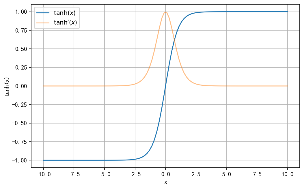
双曲正切

$$\tanh (x)=\frac{\sinh (x)}{\cosh (x)}=\frac{e^x-e^{-x}}{e^x+e^{-x}}$$

$\begin{array}{rl}{\tanh }^{\prime }(x)=& (\frac{e^x-e^{-x}}{e^x+e^{-x}}{)}^{\prime }\\ =& [(e^x-e^{-x})(e^x+e^{-x}{)}^{-1}{]}^{\prime }\\ =& (e^x+e^{-x})(e^x+e^{-x}{)}^{-1}+(e^x-e^{-x})(-1)(e^x+e^{-x}{)}^{-2}(e^x-e^{-x})\\ =& 1-(e^x-e^{-x}{)}^2(e^x+e^{-x}{)}^{-2}\\ =& 1-\frac{(e^x-e^{-x}{)}^2}{(e^x+e^{-x}{)}^2}\\ =& 1-{\tanh }^2(x)\end{array}$

def tanh(x):
    return (np.exp(x) - np.exp(-x)) / (np.exp(x) + np.exp(-x))


def d_tanh(x):
    return 1 - tanh(x)**2


x = np.linspace(-10, 10, 100)

f_x = tanh(x)

# df_x  is derivative
df_x = d_tanh(x)

plt.plot(x, f_x, label=r"$\tanh(x)}$")
plt.plot(x, df_x, label=r"$\tanh'(x)$", alpha=0.5)

plt.xlabel('x')
plt.ylabel('tanh(x)')
plt.grid()
plt.legend(loc='best')
plt.show()

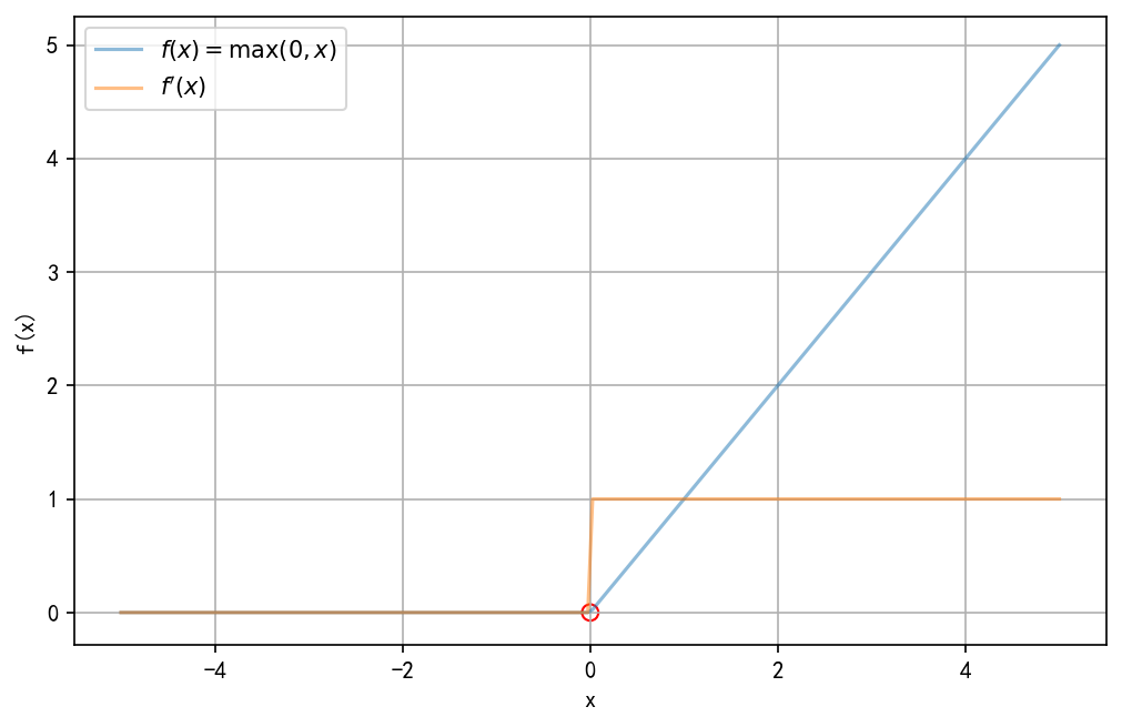
线性整流函数 rectified linear unit （ReLu）

$f(x)=\text{relu}(x)=\max (0,x)=\{\begin{array}{ll}x,& x>0\\ 0,& x\le 0\end{array}$

$f(x)是连续的$
$f^{\prime }(x)={\lim }_{h\to 0}f(0)=\frac{f(0+h)-f(0)}{h}=\frac{\max (0,h)-0}{h}$
${\lim }_{h\to 0^{-}}=\frac{0}{h}=0$
${\lim }_{h\to 0^{+}}=\frac{h}{h}=1$
所以$f^{\prime }(0)$处不可导
所以$f^{\prime }(x)=\{\begin{array}{ll}1,& x>0\\ 0,& x<0\end{array}$

$f_2=f(f(x))=max(0,f_1(x))\{\begin{array}{ll}{f}_1(x),& f_1(x)>0\\ 0,& f_1(x)\le 0\end{array}$
$\frac{d{f}_2}{dx}=\{\begin{array}{ll}1,& f_1(x)>0\\ 0,& f_1(x)\le 0\end{array}$

def relu(x):
    return np.where(x < 0, 0, x)


def d_relu(x):
    return np.where(x < 0, 0, 1)


x = np.linspace(-5, 5, 200)

f_x = relu(x)

# df_x is derivative
df_x = d_relu(x)

plt.plot(x, f_x, label=r"$ f(x) = \max(0, x)} $", alpha=0.5)
plt.plot(x, df_x, label=r"$f'(x)$", alpha=0.5)
# There is no derivative at (0)
plt.scatter(0, 0, color='', marker='o', edgecolors='r', s=50)

plt.xlabel('x')
plt.ylabel('f(x)')
plt.grid()
plt.legend()
plt.show()

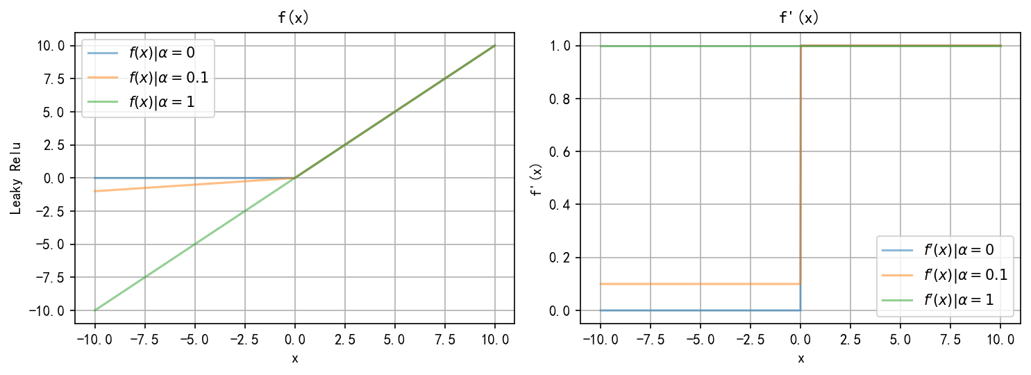
PReLU(Parametric Rectified Linear Unit) Leaky ReLu

$f(x)=\max (\alpha x,x)=\{\begin{array}{ll}x,& x>0\\ \alpha x,& x\le 0\end{array},当\alpha <1,\alpha \ne 0$,

$f(x)=\max (\alpha x,x)=\{\begin{array}{ll}\alpha x,& x>0\\ x,& x\le 0\end{array},当\alpha \ge 1$

$f(x)=\max (\alpha x,x)=\{\begin{array}{ll}x,& x>0\\ 0,& x\le 0\end{array},当\alpha =0,就是ReLu$

$当\alpha \ge 1时,f_1(x)=\{\begin{array}{ll}\alpha x,& x>0\\ x,& x\le 0\end{array}$

$\frac{d{f}_1}{dx}=\{\begin{array}{ll}\alpha ,& x>0\\ 1,& x\le 0\end{array}$

$当\alpha <1,f_1(x)=\{\begin{array}{ll}x,& x>0\\ \alpha x,& x\le 0\end{array}$

$\frac{d{f}_1}{dx}=\{\begin{array}{ll}1,& x>0\\ \alpha ,& x\le 0\end{array}$

把leaky relu的$\alpha$设置成可以训练的参数，就是PReLU(Parametric Rectified Linear Unit)

def leaky_relu(x, alpha: float = 1):
    return np.where(x <= 0, alpha * x, x)


def d_leaky_relu(x, alpha: float = 1):
    return np.where(x < 0, alpha, 1)


x = np.linspace(-10, 10, 1000)

alpha = [0, 0.1, 1]

fig, ax = plt.subplots(1, 2, figsize=(10, 3.7))

for alpha_i in alpha:
    f1 = leaky_relu(x, alpha=alpha_i)
    ax[0].plot(x, f1, label=r"$ f(x)|\alpha={0} $".format(alpha_i), alpha=0.5)
    ax[0].set_xlabel('x')
    ax[0].set_ylabel('Leaky Relu')
    ax[0].grid(True)
    ax[0].legend()
    ax[0].set_title('f(x)')

    df1 = d_leaky_relu(x, alpha_i)
    ax[1].plot(x, df1, label=r"$f'(x)|\alpha={0}$".format(alpha_i), alpha=0.5)
    ax[1].set_xlabel('x')
    ax[1].set_ylabel("f'(x)")
    ax[1].grid(True)
    ax[1].legend()
    ax[1].set_title("f'(x)")

plt.tight_layout()
plt.show()

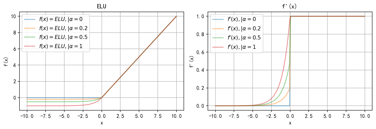
指数线性单元 Exponential Linear Units （ELU）

$f(x)=\text{elu}(x)=\{\begin{array}{ll}x,& x>0\\ \alpha (e^x-1),& x\le 0\end{array}$

$f^{\prime }(x)={\lim }_{h\to 0}f(0)=\frac{f(0+h)-f(0)}{h}$
${\lim }_{h\to 0^{-}}=\frac{\alpha (e^h-1)-0}{h}=0$
${\lim }_{h\to 0^{+}}=\frac{h}{h}=1$
所以$f^{\prime }(0)$处不可导
所以$f^{\prime }(x)=\{\begin{array}{ll}1,& x>0\\ \alpha e^x,& x\le 0\end{array}$

def elu(x, alpha: float = 1):
    return np.where(x <= 0, alpha * (np.exp(x) - 1), x)


def d_elu(x, alpha: float = 1):
    return np.where(x <= 0, alpha * np.exp(x), 1)


x = np.linspace(-10, 10, 200)

alpha = [0, 0.2, 0.5, 1]

fig, ax = plt.subplots(1, 2, figsize=(10, 3.5))
for alpha_i in alpha:
    f1 = elu(x, alpha=alpha_i)
    df1 = d_elu(x, alpha_i)
    ax[0].plot(x,
               f1,
               label=r"$f(x)=ELU,|\alpha = {0}$".format(alpha_i),
               alpha=0.5)
    ax[0].set_xlabel('x')
    ax[0].set_ylabel('f(x)')
    ax[0].grid(True)
    ax[0].legend()
    ax[0].set_title('ELU')

    ax[1].plot(x,
               df1,
               label=r"$f'(x),|\alpha = {0}$".format(alpha_i),
               alpha=0.5)
    ax[1].set_xlabel('x')
    ax[1].set_ylabel("f'(x)")
    ax[1].grid(True)
    ax[1].legend()
    ax[1].set_title("f'(x)")

plt.tight_layout()
plt.show()

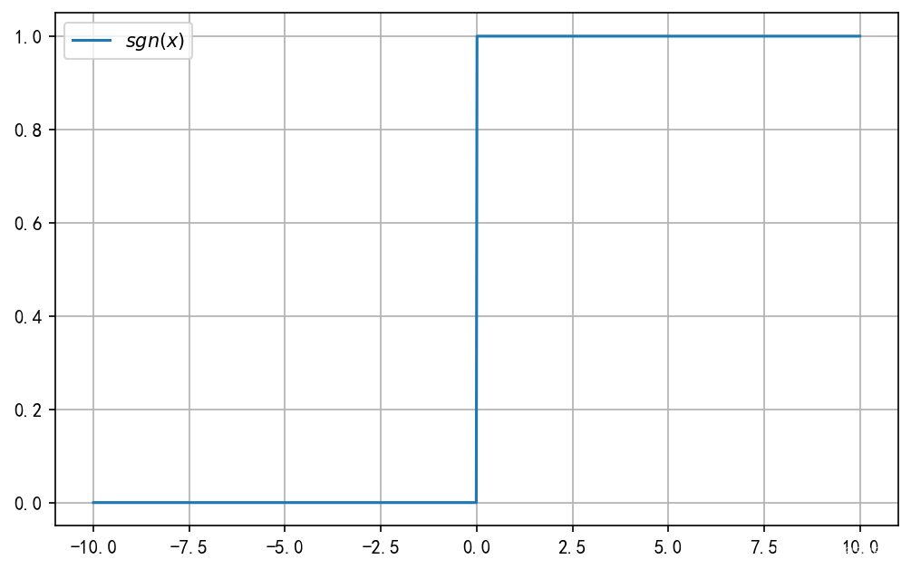
感知机激活

$\text{sgn}(x)=\{\begin{array}{ll}1,& x\ge 0\\ -1,& x<0\end{array}$

• 这里的值也可以是1，0

def sgn(x):
    return np.where(x <= 0, 0, 1)


x = np.linspace(-10, 10, 1000)

f_x = sgn(x)

plt.plot(x, f_x, label=r"$sgn(x)$", alpha=1)
plt.grid(True)
plt.legend()
plt.show()