【翻译】【SPPNet】Spatial Pyramid Pooling in Deep Convolutional Networks for Visual Recognition

Spatial Pyramid Pooling in Deep Convolutional Networks for Visual Recognition
用于视觉识别的深度卷积网络中的空间金字塔池化。

Kaiming He, Xiangyu Zhang, Shaoqing Ren, and Jian Sun

论文：https://arxiv.org/pdf/1406.4729.pdf
代码：https://github.com/ShaoqingRen/SPP_net

Abstract. Existing deep convolutional neural networks (CNNs) require afixed-size(e.g. 224×224) input image. This requirement is “artificial” and may hurt the recognition accuracy for the images or sub-images of an arbitrary size/scale. In this work, we equip the networks with a more principled pooling strategy, “spatial pyramid pooling”, to eliminate the above requirement. The new network structure, called SPP-net, can generate a fixed-length representation regardless of image size/scale. By removing the fixed-size limitation, we can improve all CNN-based image classification methods in general. Our SPP-net achieves state-ofthe-art accuracy on the datasets of ImageNet 2012, Pascal VOC 2007, and Caltech101.
摘要。现有的深度卷积神经网络（CNN）需要一个固定尺寸（如224×224）的输入图像。这种要求是 “人为的”，可能会损害任意尺寸/尺度的图像或子图像的识别精度。在这项工作中，我们为网络配备了一个更有原则的池化策略，即 “空间金字塔池化”，以消除上述要求。新的网络结构，称为SPP-net，可以生成一个固定长度的表示，而不考虑图像的大小/尺度。通过消除固定尺寸的限制，我们可以从总体上改进所有基于CNN的图像分类方法。我们的SPP-net在ImageNet 2012、Pascal VOC 2007和Caltech101的数据集上达到了最先进的准确度。
　　The power of SPP-net is more significant in object detection. Using SPP-net, we compute the feature maps from the entire image only once, and then pool features in arbitrary regions (sub-images) to generate fixed-length representations for training the detectors. This method avoids repeatedly computing the convolutional features. In processing test images, our method computes convolutional features 30-170× faster than the recent leading method R-CNN (and 24-64× faster overall), while achieving better or comparable accuracy on Pascal VOC 2007(A longer technical report of our paper is in http://arxiv.org/abs/1406.4729v1.pdf).
　　在目标检测中，SPP-net的力量更为显著。使用SPP-net，我们只需从整个图像中计算一次特征图，然后在任意区域（子图像）中汇集特征，生成固定长度的表示，用于训练检测器。这种方法避免了重复计算卷积特征。在处理测试图像时，我们的方法计算卷积特征的速度比最近领先的方法R-CNN快30-170倍（总体上快24-64倍），同时在Pascal VOC 2007上取得更好或相当的准确性（我们论文的较长技术报告在http://arxiv.org/abs/1406.4729v1.pdf）。

1 Introduction（介绍）

We are witnessing a rapid, revolutionary change in our vision community, mainly caused by deep convolutional neural networks (CNNs) [18] and the availability of large scale training data [6]. Deep-networks-based approaches have recently been substantially improving upon the state of the art in image classification [16,31,24], object detection [12,33,24], many other recognition tasks [22,27,32,13], and even non-recognition tasks.
　　我们正在见证视觉界的快速、革命性的变化，主要是由深度卷积神经网络（CNN）[18]和大规模训练数据的可用性[6]引起的。基于深度网络的方法最近在图像分类[16,31,24]、目标检测[12,33,24]、许多其他识别任务[22,27,32,13]，甚至非识别任务方面的技术水平上有了很大提高。

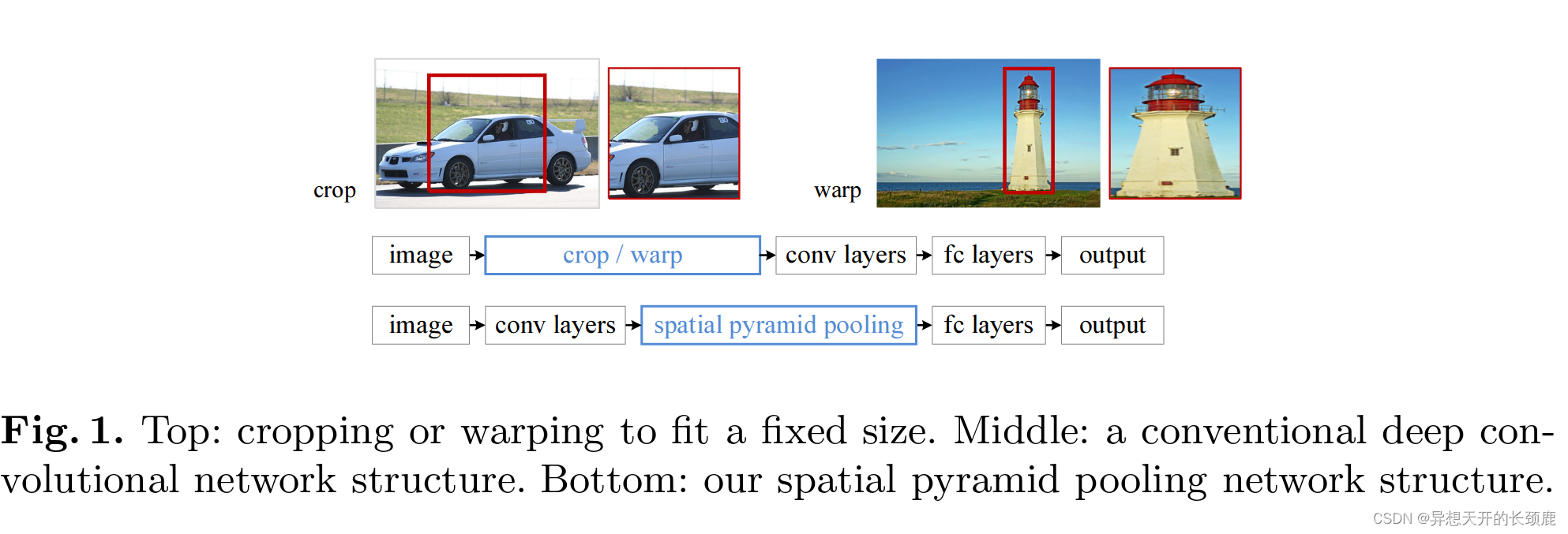
　　However, there is a technical issue in the training and testing of the CNNs: the prevalent CNNs require a fixed input image size (e.g., 224×224), which limits both the aspect ratio and the scale of the input image. When applied to images of arbitrary sizes, current methods mostly fit the input image to the fixed size, either via cropping [16,31] or via warping [7,12], as shown in Fig. 1 (top). But the cropped region may not contain the entire object, while the warped content may result in unwanted geometric distortion. Recognition accuracy can be compromised due to the content loss or distortion. Besides, a pre-defined scale (e.g., 224) may not be suitable when object scales vary. Fixing the input size overlooks the issues involving scales.
　　然而，在CNN的训练和测试中存在一个技术问题：主流的CNN需要一个固定的输入图像尺寸（例如224×224），这就限制了输入图像的长宽比和比例。当应用于任意尺寸的图像时，目前的方法大多通过裁剪[16,31]或通过扭曲[7,12]将输入的图像适合于固定的尺寸，如图1（顶部）所示。但是，裁剪的区域可能不包含整个物体，而扭曲的内容可能导致不必要的几何变形。由于内容的损失或扭曲，识别精度可能会受到影响。此外，当目标的尺度变化时，预先定义的尺度（如224）可能并不适合。固定的输入尺寸忽略了涉及尺度的问题。

　　So why do CNNs require a fixed input size? A CNN mainly consists of two parts: convolutional layers, and fully-connected layers that follow. The convolutional layers operate in a sliding-window manner and output feature maps which represent the spatial arrangement of the activations (Fig. 2). In fact, convolutional layers do not require a fixed image size and can generate feature maps of any sizes. On the other hand, the fully-connected layers need to have fixedsize/length input by their definition. Hence, the fixed-size constraint comes only from the fully-connected layers, which exist at a deeper stage of the network.
　　那么，为什么CNN需要一个固定的输入大小呢？一个CNN主要由两部分组成：卷积层和后面的全连接层。卷积层以滑动窗口的方式运行，并输出代表激活的空间排列的特征图（图2）。事实上，卷积层不需要固定的图像尺寸，可以生成任何尺寸的特征图。另一方面，全连接层根据其定义需要有固定大小/长度的输入。因此，固定尺寸的约束只来自全连接层，它存在于网络的较深阶段。
　　In this paper, we introduce a spatial pyramid pooling (SPP) [14,17] layer to remove the fixed-size constraint of the network. Specifically, we add an SPP layer on top of the last convolutional layer. The SPP layer pools the features and generates fixed-length outputs, which are then fed into the fully-connected layers (or other classifiers). In other words, we perform some information “aggregation” at a deeper stage of the network hierarchy (between convolutional layers and fully-connected layers) to avoid the need for cropping or warping at the beginning. Fig. 1 (bottom) shows the change of the network architecture by introducing the SPP layer. We call the new network structure SPP-net.
　　在本文中，我们引入了一个空间金字塔池化（SPP）[14,17]层来消除网络的固定尺寸约束。具体来说，我们在最后一个卷积层的顶部添加一个SPP层。SPP层汇集特征并产生固定长度的输出，然后将其送入全连接层（或其他分类器）。换句话说，我们在网络层次结构的较深阶段（卷积层和全连接层之间）进行一些信息 “聚合”，以避免一开始就进行裁剪或扭曲。图1（底部）显示了引入SPP层后网络结构的变化。我们称这种新的网络结构为SPP-net。
　　We believe that aggregation at a deeper stage is more physiologically sound and more compatible with the hierarchical information processing in our brains. When an object comes into our field of view, it is more reasonable that our brains consider it as a whole instead of cropping it into several “views” at the beginning. Similarly, it is unlikely that our brains distort all object candidates into fixed-size regions for detecting/locating them. It is more likely that our brains handle arbitrarily-shaped objects at some deeper layers, by aggregating the already deeply processed information from the previous layers.
　　我们认为，在更深的阶段进行聚合，在生理上更合理，也更符合我们大脑中的信息处理层次结构。当一个物体进入我们的视野时，我们的大脑将其视为一个整体，而不是一开始就将其裁剪成几个 “视图”，这是比较合理的。同样，我们的大脑也不可能将所有候选物体扭曲成固定大小的区域来检测/定位它们。更有可能的是，我们的大脑在一些更深的层次上处理任意形状的物体，通过聚合前几层已经深入处理的信息。
　　Spatial pyramid pooling [14,17] (popularly known as spatial pyramid matching or SPM [17]), as an extension of the Bag-of-Words (BoW) model [25], is one of the most successful methods in computer vision. It partitions the image into divisions from finer to coarser levels, and aggregates local features in them. SPP has long been a key component in the leading and competition-winning systems for classification (e.g., [30,28,21]) and detection (e.g., [23]) before the recent prevalence of CNNs. Nevertheless, SPP has not been considered in the context of CNNs. We note that SPP has several remarkable properties for deep CNNs: 1) SPP is able to generate a fixed-length output regardless of the input size, while the sliding window pooling used in the previous deep networks [16] cannot; 2) SPP uses multi-level spatial bins, while the sliding window pooling uses only a single window size. Multi-level pooling has been shown to be robust to object deformations [17]; 3) SPP can pool features extracted at variable scales thanks to the flexibility of input scales. Through experiments we show that all these factors elevate the recognition accuracy of deep networks.
　　空间金字塔池化[14,17]（俗称空间金字塔匹配或SPM[17]），作为Bag-of-Words（BoW）模型[25]的延伸，是计算机视觉中最成功的方法之一。它将图像划分为从细到粗的层次，并将局部特征聚集在其中。在最近CNN盛行之前，SPP长期以来一直是分类（如[30,28,21]）和检测（如[23]）的领先和竞赛获奖系统的关键组成部分。然而，SPP还没有在CNN的背景下被考虑。我们注意到，SPP对于深度CNN来说有几个显著的特性。1）SPP能够产生一个固定长度的输出，而之前的深度网络中使用的滑动窗池化[16]则不能；2）SPP使用多级空间仓，而滑动窗池化只使用一个窗口大小。多级池化已被证明对目标变形具有鲁棒性[17]；3）由于输入尺度的灵活性，SPP可以汇集在不同尺度上提取的特征。通过实验我们表明，所有这些因素都提升了深度网络的识别精度。
　　The flexibility of SPP-net makes it possible to generate a full-image representation for testing. Moreover, it also allows us to feed images with varying sizes or scales during training, which increases scale-invariance and reduces the risk of over-fitting. We develop a simple multi-size training method to exploit the properties of SPP-net. Through a series of controlled experiments, we demonstrate the gains of using multi-level pooling, full-image representations, and variable scales. On the ImageNet 2012 dataset, our network reduces the top-1 error by 1.8% compared to its counterpart without SPP. The fixed-length representations given by this pre-trained network are also used to train SVM classifiers on other datasets. Our method achieves 91.4% accuracy on Caltech101 [9] and 80.1% mean Average Precision (mAP) on Pascal VOC 2007 [8] using only a single full-image representation (single-view testing).
　　SPP-net的灵活性使其有可能在测试中生成一个完整的图像表示。此外，它还允许我们在训练过程中输入不同大小或比例的图像，这增加了尺度不变性并降低了过度拟合的风险。我们开发了一种简单的多尺寸训练方法来利用SPP-net的特性。通过一系列的控制性实验，我们证明了使用多级池化、全图像表示和可变尺度的好处。在ImageNet 2012数据集上，与没有SPP的对应网络相比，我们的网络将top-1的错误降低了1.8%。这个预训练的网络所给出的固定长度的表示也被用来在其他数据集上训练SVM分类器。我们的方法在Caltech101[9]上取得了91.4%的准确率，在Pascal VOC 2007[8]上仅使用单一的全图像表示（单视图测试）取得了80.1%的平均精度（mAP）。
　　SPP-net shows even greater strength in object detection. In the leading object detection method R-CNN [12], the features from candidate windows are extracted via deep convolutional networks. This method shows remarkable detection accuracy on both the VOC and ImageNet datasets. But the feature computation in R-CNN is time-consuming, because it repeatedly applies the deep convolutional networks to the raw pixels of thousands of warped regions per image. In this paper, we show that we can run the convolutional layers only once on the entire image (regardless of the number of windows), and then extract features by SPP-net on the feature maps. This method yields a speedup of over one hundred times over R-CNN. Note that training/running a detector on the feature maps (rather than image regions) is actually a more popular idea [10,5,23,24]. But SPP-net inherits the power of the deep CNN feature maps and also the flexibility of SPP on arbitrary window sizes, which leads to outstanding accuracy and efficiency. In our experiment, the SPP-net-based system (built upon the R-CNN pipeline) computes convolutional features 30-170× faster than R-CNN, and is overall 24-64× faster, while has better or comparable accuracy. We further propose a simple model combination method to achieve a new stateof-the-art result (mAP 60.9%) on the Pascal VOC 2007 detection task.
　　SPP-net在目标检测方面显示出更大的优势。在领先的目标检测方法R-CNN[12]中，候选窗口的特征是通过深度卷积网络提取的。这种方法在VOC和ImageNet数据集上都显示出显著的检测精度。但是R-CNN中的特征计算是很耗时的，因为它将深度卷积网络反复应用于每幅图像的数千个扭曲region的原始像素。在本文中，我们表明我们可以在整个图像上只运行一次卷积层（不管窗口的数量如何），然后通过SPP-net在特征图上提取特征。这种方法产生的速度比R-CNN快一百多倍。请注意，在特征图（而不是图像区域）上训练/运行检测器实际上是一个更流行的想法[10,5,23,24]。但是SPP-net继承了深度CNN特征图的力量，同时也继承了SPP在任意窗口大小上的灵活性，这就导致了杰出的准确性和效率。在我们的实验中，基于SPP-net的系统（建立在R-CNN管道上）计算卷积特征的速度比R-CNN快30-170倍，总体上快24-64倍，同时具有更好或相当的准确性。我们进一步提出了一个简单的模型组合方法，在Pascal VOC 2007检测任务中取得了新的最先进的结果（mAP 60.9%）。

2 Deep Networks with Spatial Pyramid Pooling（带有空间金字塔池化的深度网络）

2.1 Convolutional Layers and Feature Maps（卷积层和特征图）

Consider the popular seven-layer architectures [16,31]. The first five layers are convolutional, some of which are followed by pooling layers. These pooling layers can also be considered as “convolutional”, in the sense that they are using sliding windows. The last two layers are fully connected, with an N-way softmax as the output, where N is the number of categories.
　　考虑一下主流的七层架构[16,31]。前五层是卷积层，其中一些之后是池化层。这些池化层也可以被认为是 “卷积”，因为它们使用的是滑动窗口。最后两层是全连接的，输出是N-way softmax，其中N是类别的数量。
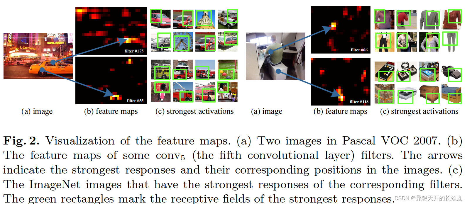
　　The deep network described above needs a fixed image size. However, we notice the requirement of fixed sizes is only due to the fully-connected layers that demand fixed-length vectors as inputs. On the other hand, the convolutional layers accept inputs of arbitrary sizes. The convolutional layers use sliding filters, and their outputs have roughly the same aspect ratio as the inputs. These outputs are known as feature maps [18] - they involve not only the strength of the responses, but also their spatial positions. In Fig. 2, we visualize some feature maps. They are generated by some filters of the $con{v}_5$ layer.
　　上面描述的深度网络需要一个固定的图像尺寸。然而，我们注意到对固定尺寸的要求只是由于全连接层需要固定长度的向量作为输入。另一方面，卷积层接受任意大小的输入。卷积层使用滑动滤波器，其输出与输入的长宽比大致相同。这些输出被称为特征图[18]–它们不仅涉及反应的强度，还涉及它们的空间位置。在图2中，我们可视化了一些特征图。它们是由$con{v}_5$层的一些过滤器生成的。
　　It is worth noticing that we generate the feature maps in Fig. 2 without fixing the input size. These feature maps generated by deep convolutional layers are analogous to the feature maps in traditional methods [2,4]. In those methods, SIFT vectors [2] or image patches [4] are densely extracted and then encoded, e.g., by vector quantization [25,17,11], sparse coding [30,28], or Fisher kernels [21]. These encoded features consist of the feature maps, and are then pooled by Bag-of-Words (BoW) [25] or spatial pyramids [14,17]. Analogously, the deep convolutional features can be pooled in a similar way.
　　值得注意的是，我们在图2中生成的特征图没有固定输入大小。这些由深度卷积层生成的特征图类似于传统方法中的特征图[2,4]。在这些方法中，SIFT向量[2]或图像patches[4]被密集提取，然后进行编码，例如，通过向量量化[25,17,11]、稀疏编码[30,28]或Fisher核[21]。这些编码后的特征由特征图组成，然后通过词袋（BoW）[25]或空间金字塔[14,17]进行汇集。类似地，深度卷积特征也可以用类似的方式进行汇集。

2.2 The Spatial Pyramid Pooling Layer（空间金字塔池化层）

The convolutional layers accept arbitrary input sizes, but they produce outputs of variable sizes. The classifiers (SVM/softmax) or fully-connected layers require fixed-length vectors. Such vectors can be generated by the Bag-of-Words (BoW) approach [25] that pools the features together. Spatial pyramid pooling [14,17] improves BoW in that it can maintain spatial information by pooling in local spatial bins. These spatial bins have sizes proportional to the image size, so the number of bins is fixed regardless of the image size. This is in contrast to the sliding window pooling of the previous deep networks [16], where the number of sliding windows depends on the input size.
　　卷积层接受任意大小的输入，但它们产生的输出是可变大小的。分类器（SVM/softmax）或全连接层需要固定长度的向量。这种向量可以通过将特征汇集在一起的Bag-of-Words（BoW）方法[25]产生。空间金字塔池化[14,17]改进了BoW，因为它可以通过在局部空间仓中集合来保持空间信息。这些空间仓的大小与图像大小成正比，因此无论图像大小如何，仓的数量是固定的。这与之前的深度网络的滑动窗口池形成对比[16]，滑动窗口的数量取决于输入大小。
　　To adopt the deep network for images of arbitrary sizes, we replace the $poo{l}_5$ layer (the pooling layer after $con{v}_5$)withaspatial pyramid pooling layer.Fig.3 illustrates our method. In each spatial bin, we pool the responses of each filter (throughout this paper we use max pooling). The outputs of SPP are 256M-d vectors with the number of bins denoted as M (256 is the number of $con{v}_5$ filters). The fixed-dimensional vectors are the input to the fc layer ($f{c}_6$).
　　为了对任意尺寸的图像采用深度网络，我们用空间金字塔池化层取代$poo{l}_5$层（$con{v}_5$之后的池化层）。在每个空间仓中，我们将每个滤波器的响应集合起来（本文中我们使用最大池化）。SPP的输出是256M-d向量，bin的数量表示为M（256是$con{v}_5$滤波器的数量）。固定维度的向量是fc层（$f{c}_6$）的输入。
　　With SPP, the input image can be of any sizes; this not only allows arbitrary aspect ratios, but also allows arbitrary scales. We can resize the input image to any scale (e.g., min(w, h)=180, 224, …) and apply the same deep network. When the input image is at different scales, the network (with the same filter sizes) will extract features at different scales. The scales play important roles in traditional methods, e.g., the SIFT vectors are often extracted at multiple scales [19,2] (determined by the sizes of the patches and Gaussian filters). We will show that the scales are also important for the accuracy of deep networks.
　　使用SPP，输入的图像可以是任何尺寸；这不仅允许任意的长宽比，还允许任意的比例。我们可以将输入图像的大小调整为任何尺度（例如，min(w, h)=180, 224, …），并应用相同的深度网络。当输入图像处于不同尺度时，网络（具有相同的过滤器大小）将提取不同尺度的特征。尺度在传统方法中起着重要的作用，例如，SIFT向量通常是在多个尺度上提取的[19,2]（由patches和高斯滤波器的大小决定）。我们将表明，尺度对深度网络的准确性也很重要。

2.3 Training the Network with the Spatial Pyramid Pooling Layer（带有空间金字塔池化的网络训练）

Theoretically, the above network structure can be trained with standard backpropagation [18], regardless of the input image size. But in practice the GPU implementations (such as convnet [16] and Caffe [7]) are preferably run on fixed input images. Next we describe our training solution that takes advantage of these GPU implementations while still preserving the SPP behaviors.
　　理论上，上述网络结构可以用标准的反向传播法[18]来训练，而不考虑输入图像的大小。但在实践中，GPU的实现（如convnet[16]和Caffe[7]）最好是在固定的输入图像上运行。接下来我们将介绍我们的训练方案，该方案利用了这些GPU实现，同时仍然保留了SPP行为。

　　Single-Size Training. As in previous works, we first consider a network taking a fixed-size input ($224\times 224$) cropped from images. The cropping is for the purpose of data augmentation. For an image with a given size, we can pre-compute the bin sizes needed for spatial pyramid pooling. Consider the feature maps after $con{v}_5$ that have a size of $a\times a$ (e.g.,$13\times 13$). 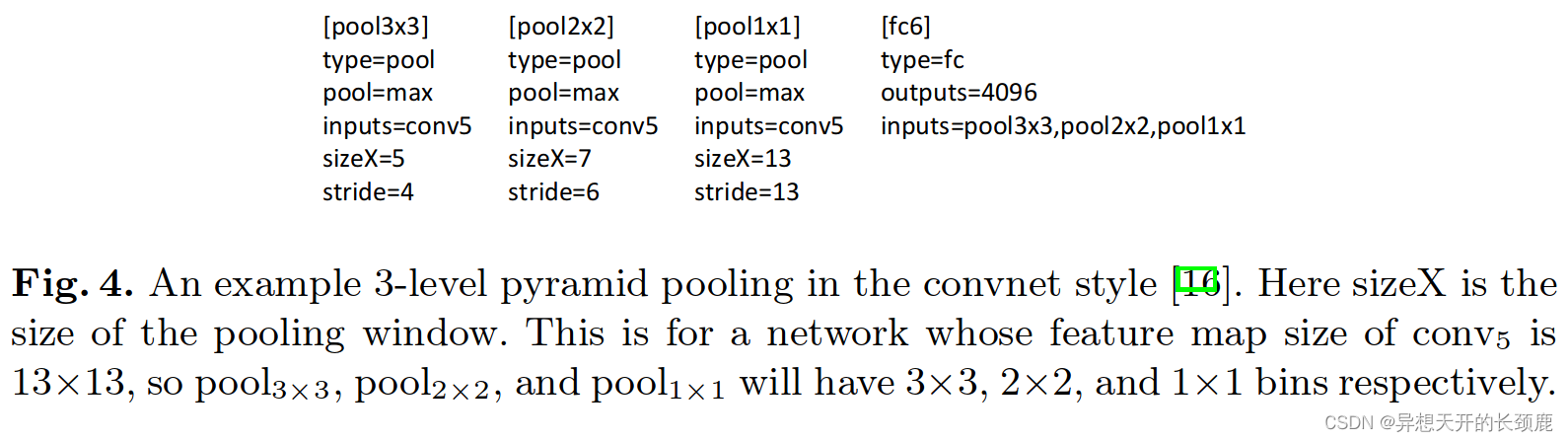With a pyramid level of n×n bins, we implement this pooling level as a sliding window pooling, where the window size $win=\lceil a/n\rceil$ and stride $str=\lfloor a/n\rfloor$ with $\lceil \cdot \rceil$ and $\lfloor \cdot \rfloor$ denoting ceiling and floor operations. With an l-level pyramid, we implement l such layers. The next fc layer (fc6) will concatenate the l outputs. Fig. 4 shows an example configuration of 3-level pyramid pooling (3×3, 2×2, 1×1) in the convnet style [16].
　　单一尺寸训练。和以前的工作一样，我们首先考虑一个网络从图像中获取一个固定大小的输入（224×224）。裁剪的目的是为了增加数据。对于一个给定尺寸的图像，我们可以预先计算出空间金字塔池所需的bin尺寸。考虑到$con{v}_5$之后的特征图，其大小为$a\times a$（例如，$13\times 13$）。对于n×n个bin的金字塔级别，我们将这个池化级别作为滑动窗口池化来实现，其中窗口大小$win=\lceil a/n\rceil$，$str=\lfloor a/n\rfloor$，其中$\lceil \cdot \rceil$和$\lfloor \cdot \rfloor$表示向上取整和向下取整操作。在一个l级金字塔中，我们实现了l个这样的层。下一个fc层（fc6）将把l个输出连接起来。图4显示了一个3级金字塔池（3×3，2×2，1×1）在convnet风格中的配置实例[16]。
　　The main purpose of our single-size training is to enable the multi-level pooling behavior. Experiments show that this is one reason for the gain of accuracy.
　　我们进行单一尺寸训练的主要目的是为了实现多层次的池化行为。实验表明，这是准确性提高的一个原因。
　　Multi-size Training. Our network with SPP is expected to be applied on images of any sizes. To address the issue of varying image sizes in training, we consider a set of pre-defined sizes. We use two sizes (180×180 in addition to 224×224) in this paper. Rather than crop a smaller 180×180 region, we resize the aforementioned 224×224 region to 180×180. So the regions at both scales differ only in resolution but not in content/layout. For the network to accept 180×180 inputs, we implement another fixed-size-input (180×180) network. The feature map size after conv5 is a×a =10×10 in this case. Then we still use $win=\lceil a/n\rceil$ and $str=\lfloor a/n\rfloor$ to implement each pyramid level. The output of the SPP layer of this 180-network has the same fixed length as the 224-network. As such, this 180-network has exactly the same parameters as the 224-network in each layer. In other words, during training we implement the varying-size-input SPP-net by two fixed-size-input networks that share parameters.
　　多尺寸训练。我们的网络与SPP预计将应用于任何尺寸的图像。为了解决训练中不同图像尺寸的问题，我们考虑了一组预先确定的尺寸。我们在本文中使用了两种尺寸（除224×224外，还有180×180）。我们没有裁剪一个较小的180×180区域，而是将上述224×224区域的大小调整为180×180。因此，两种比例的区域只在分辨率上有区别，而在内容/布局上没有区别。为了让网络接受180×180的输入，我们实现了另一个固定大小的输入（180×180）网络。在这种情况下，conv5之后的特征图大小为a×a=10×10。然后我们仍然使用$win=\lceil a/n\rceil$和$str=\lfloor a/n\rfloor$来实现每个金字塔层。这个180网络的SPP层的输出与224网络的固定长度相同。因此，这个180×180网络的每一层的参数与224×224网络的参数完全相同。换句话说，在训练过程中，我们通过两个共享参数的固定大小的输入网络来实现可变大小的SPP网络。
　　To reduce the overhead to switch from one network (e.g., 224) to the other (e.g., 180), we train each full epoch on one network, and then switch to the other one (copying all weights) for the next full epoch. This is iterated. In experiments, we find the convergence rate of this multi-size training to be similar to the above single-size training. We train 70 epochs in total as is a common practice.
　　为了减少从一个网络（如224）切换到另一个网络（如180）的开销，我们在一个网络上训练每个完整的epoch，然后切换到另一个网络（复制所有权重）进行下一个完整的epoch。这样反复进行。在实验中，我们发现这种多尺寸训练的收敛率与上述单尺寸训练相似。我们总共训练了70个epochs，这是一个常见的做法。
　　The main purpose of multi-size training is to simulate the varying input sizes while still leveraging the existing well-optimized fixed-size implementations. In theory, we could use more scales/aspect ratios, with one network for each scale/aspect ratio and all networks sharing weights, or we could develop a varying-size implementation to avoid switching. We will study this in the future. Note that the above single/multi-size solutions are for training only. At the testing stage, it is straightforward to apply SPP-net on images of any sizes.
　　多尺寸训练的主要目的是模拟不同的输入尺寸，同时仍然利用现有的经过优化的固定尺寸实现。理论上，我们可以使用更多的尺度/角度比率，每个尺度/角度比率有一个网络，所有的网络共享权重，或者我们可以开发一个不同大小的实现来避免切换。我们将在未来研究这个问题。请注意，上述单/多尺寸的解决方案仅用于训练。在测试阶段，在任何尺寸的图像上应用SPP-net都是直接的。

3 SPP-Net for Image Classification （用于图像分类的SPP-Net）

3.1 Experiments on ImageNet 2012 Classification（ImageNet 2012分类实验）

We trained our network on the 1000-category training set of ImageNet 2012. Our training details follow the practices of previous work [16,31,15]. The images are resized so that the smaller dimension is 256, and a 224×224 crop is picked from the center or the four corners from the entire image(In [16], the four corners are picked from the corners of the central 256×256 crop.). The data are augmented by horizontal flipping and color altering [16]. Dropout [16] is used on the two fully-connected layers. The learning rate starts from 0.01, and is divided by 10 (twice) when the error plateaus. Our implementation is based on the publicly available code of convnet [16]. Our experiments are run on a GTX Titan GPU.
　　我们在ImageNet 2012的1000个类别的训练集上训练我们的网络。我们的训练细节遵循了以前工作的惯例[16,31,15]。我们调整了图像的大小，使其较小的维度为256，并从整个图像的中心或四个角中挑选出224×224的裁剪（在[16]中，四个角是从中央256×256的裁剪中挑选出来的）。这些数据通过水平翻转和颜色改变来增加[16]。在两个全连接层上使用了Dropout[16]。学习率从0.01开始，当误差达到峰值时再除以10（两次）。我们的实现是基于convnet[16]的公开可用代码。我们的实验是在GTX Titan GPU上运行的。

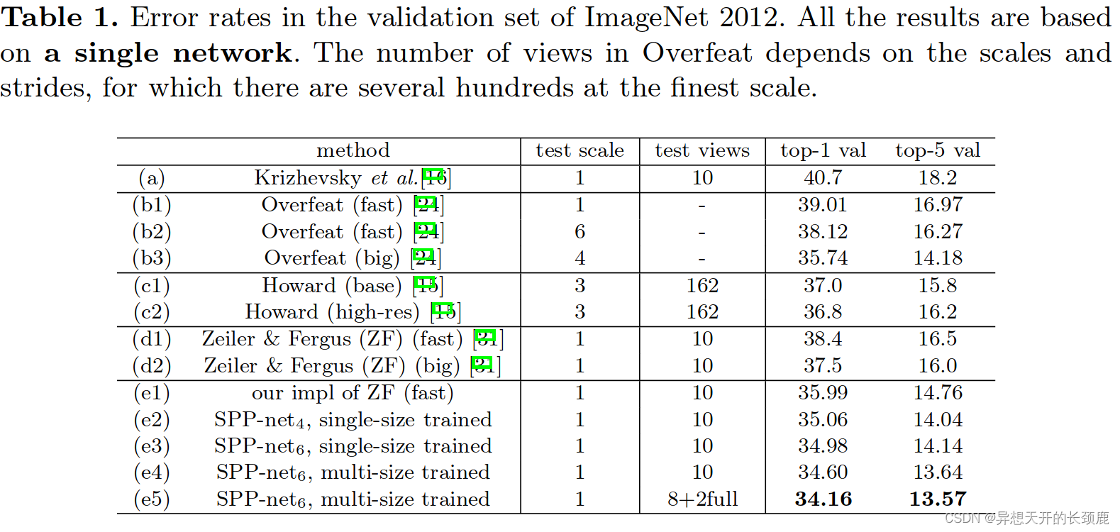
　　As our baseline model, we implement the 7-layer network of Zeiler and Fergus’s (ZF) “fast” (smaller) model [31], which produces competitive results with a moderate training time (two weeks). The filter numbers (sizes) of the five convolutional layers are: 96(7 × 7), 256(5 × 5), 384(3 × 3), 384(3 × 3), and 256(3 × 3). The first two layers have a stride of 2, and the rest have a stride of 1.The first two layers are followed by (sliding window) max pooling with a stride of 2, window size of 3, and contrast normalization operations. The outputs of the two fully-connected layers are 4096-d. At the testing stage, we follow the standard 10-view prediction in [16]: each view is a 224×224 crop and their scores are averaged. Our replication of this network gives 35.99% top-1 error (Tab. 1 (e1)), better than 38.4% (Tab. 1 (d1)) as reported in [31]. We believe this margin is because the corner crops are from the entire image (rather than from the corners of the central 256×256 square), as is reported in [15].
　　作为我们的基线模型，我们实现了Zeiler和Fergus（ZF）的 “fast”（较小）模型的7层网络[31]，它在适度的训练时间（两周）内产生了有竞争力的结果。五个卷积层的过滤器数量（大小）是。96（7×7），256（5×5），384（3×3），384（3×3）和256（3×3）。前两层的步长为2，其余的步长为1。前两层之后是（滑动窗口）最大池化，跨度为2，窗口大小为3，以及对比度归一化操作。两个全连接层的输出为4096-d。在测试阶段，我们遵循[16]中标准的10个视图预测：每个视图是一个224×224的裁剪，它们的分数是平均的。我们对这个网络的复制给出了35.99%的top-1误差（表1（e1）），优于[31]中报告的38.4%（表1（d1））。我们认为这个幅度是因为角部的裁剪来自整个图像（而不是像[15]中报告的那样来自中央256×256方块的角部）。
　　Tab. 1 (e2)(e3) show our results using single-size training. The training and testing sizes are both 224×224. In these networks, the convolutional layers have the same structures as the ZF fast model, whereas the pooling layer after conv5 is replaced with the SPP layer. We use a 4-level pyramid. The pyramid is {4×4, 3×3, 2×2, 1×1}, totally 30 bins and denoted as SPP-net4 (e2), or {6×6, 3×3, 2×2, 1×1}, totally 50 bins and denoted as SPP-net6 (e3). In these results, we use 10-view prediction with each view a 224×224 crop. The top-1 error of SPPnet4 is 35.06%, and of SPP-net6 is 34.98%. These results show considerable improvement over the no-SPP counterpart (e1). Since we are still using the same 10 cropped views as in (e1), this gain is solely because of multi-level pooling. Note that SPP-net4 has even fewer parameters than the no-SPP model (fc6 has 30×256-d inputs instead of 36×256-d). So the gain of the multi-level pooling is not simply due to more parameters. Rather, it is because the multi-level pooling is robust to the variance in object deformations and spatial layout [17].
　　Tab. 1(e2)(e3)显示了我们使用单一尺寸训练的结果。训练和测试尺寸都是224×224。在这些网络中，卷积层的结构与ZF的fast模型相同，而conv5之后的池化层被SPP层取代。我们使用一个4级金字塔。该金字塔为{4×4, 3×3, 2×2, 1×1}，共30个bin，表示为SPP-net4（e2），或{6×6, 3×3, 2×2, 1×1}，共50个bin，表示为SPP-net6（e3）。在这些结果中，我们使用10个视图的预测，每个视图为224×224的裁剪。SPPnet4的Top-1误差为35.06%，SPP-net6为34.98%。这些结果显示出比无SPP的对应方案（e1）有相当大的改进。由于我们仍然使用与(e1)相同的10个裁剪过的视图，这种改进完全是由于多级池化的作用。请注意，SPP-net4的参数甚至比无SPP模型更少（fc6有30×256-d的输入而不是36×256-d）。因此，多级池化的收益并不仅仅是由于更多的参数。相反，这是因为多级池化对物体变形和空间布局的差异具有鲁棒性[17]。
　　Tab. 1 (e4) shows our result using multi-size training. The training sizes are 224 and 180, while the testing size is still 224. In (e4) we still use the 10 cropped views for prediction. The top-1 error drops to 34.60%. Note the networks in (e3) and (e4) have exactly the same structure and the same method for testing. So the gain is solely because of the multi-size training.
　　Tab. 1（e4）显示了我们使用多尺寸训练的结果。训练尺寸为224和180，而测试尺寸仍为224。在（e4）中，我们仍然使用10个裁剪过的视图进行预测。Top-1的误差下降到34.60%。注意（e3）和（e4）中的网络有完全相同的结构和相同的测试方法。所以收益完全是由于多尺寸训练。
　　Next we investigate the accuracy of the full-image views. We resize the image so that $min(w,h)=256$ while maintaining its aspect ratio. The SPP-net is applied on this full image to compute the scores of the full view. For fair comparison, we also evaluate the accuracy of the single view in the center 224×224 crop (which is used in the above evaluations). The comparisons of single-view testing accuracy are in Tab. 2. The top-1 error rates are reduced by about 0.5%. This shows the importance of maintaining the complete content. Even though our network is trained using square images only, it generalizes well to other aspect ratios.
　　接下来我们调查整图的准确性。我们调整图像的大小，使$min(w,h)=256$，同时保持其长宽比。SPP-net被应用在这个整图上，以计算整图的分数。为了公平比较，我们也评估了中间224×224裁剪的单视图的准确性（在上述评估中使用）。单视图测试精度的比较见表2。top-1的错误率降低了约0.5%。这表明保持完整内容的重要性。尽管我们的网络只用方形图像进行训练，但它对其他长宽比的图像有很好的概括性。
　　In Tab. 1 (e5), we replace the two center cropped views with two full-views (with flipping) for testing. The top-1 error is further reduced to 34.16%. This again indicates that the full-image views are more representative than the cropped views(However, the combination of the 8 cropped views is still useful.). The SPP-net in (e5) is better than the no-SPP counterpart (e1) by 1.8%.
　　在Tab. 1(e5)中，我们用两个全视野(翻转)来代替两个中间裁剪的视图进行测试。top-1的误差进一步减少到34.16%。这再次表明全图视图比剪裁后的视图更具代表性（然而，8个剪裁后的视图的组合仍然是有用的）。(e5)中的SPP-网络比无SPP的对照(e1)好1.8%。
　　There are previous CNN solutions [24,15] that deal with various scales/sizes, but they are based on model averaging. In Overfeat [24] and Howard’s method [15], the single network is applied at multiple scales in the testing stage, and the scores are averaged. Howard further trains two different networks on low/highresolution image regions and averages the scores. These methods generate much more views (e.g., over hundreds), but the sizes of the views are still pre-defined beforehand. On the contrary, our method builds the SPP structure into the network, and uses multi-size images to train a single network. Our method also enables the use of full-view as a single image representation.
　　以前有一些CNN解决方案[24,15]处理各种尺度/尺寸，但它们是基于模型的平均化。在Overfeat[24]和Howard的方法[15]中，单一网络在测试阶段被应用于多个尺度，并对得分进行平均。Howard在低/高分辨率的图像区域进一步训练两个不同的网络，并对分数进行平均。这些方法产生的视图要多得多（例如，超过数百个），但视图的大小仍然是事先预设的。相反，我们的方法在网络中建立了SPP结构，并使用多尺寸图像来训练一个网络。我们的方法还能够使用全视图作为单一的图像表示。
　　Our results can be potentially improved further. The usage of the SPP layer does not depend on the design of the convolutional layers. So our method may benefit from, e.g., increased filter numbers or smaller strides [31,24]. Multiplemodel averaging also may be applied. We will study these in the future.
　　我们的结果有可能被进一步改进。SPP层的使用并不取决于卷积层的设计。因此，我们的方法可能会受益于，例如，增加过滤器数量或缩小步幅[31,24]。多模型平均法也可以应用。我们将在未来研究这些。

3.2 Experiments on Pascal VOC 2007 Classification（Pascal VOC 2007分类实验）

With the networks pre-trained on ImageNet, we extract representations from the images in other datasets and re-train SVM classifiers [1] for the new datasets. In the SVM training, we intentionally do not use any data augmentation (flip/multiview). We l2-normalize the features and fix the SVM’s soft margin parameter C to 1. We use our multi-size trained model in Tab. 1 (e5).
　　通过在ImageNet上预训练的网络，我们从其他数据集的图像中提取表征，并为新的数据集重新训练SVM分类器[1]。在SVM训练中，我们有意不使用任何数据增强（翻转/多视图）。我们对特征进行l2归一化，并将SVM的软边际参数C固定为1。我们在表1（e5）中使用了我们的多尺寸训练模型。

　　The classification task in Pascal VOC 2007 [8] involves 9,963 images in 20 categories. 5,011 images are for training, and the rest are for testing. The performance is evaluated by mAP. Tab. 3 summarizes our results for different settings.
　　Pascal VOC 2007[8]的分类任务涉及20个类别的9,963张图像。5,011张图像用于训练，其余的用于测试。性能是由mAP来评估的。表3总结了我们在不同设置下的结果。
　　We start from a baseline in Tab. 3 (a). The model is the one in Tab. 1 (e1) without SPP (“plain net”). To apply this model, we resize the image so that min(w, h) = 224, and crop the center 224×224 region. The SVM is trained via the features of a layer. On this dataset, the deeper the layer is, the better the result is. In col.(b), we replace the plain net with our SPP-net. As a first-step comparison, we still apply the SPP-net on the center 224×224 crop. The results of the fc layers improve. This gain is mainly due to multi-level pooling.
　　我们从表3（a）的基线开始。该模型是表1（e1）中没有SPP的模型（“普通网”）。为了应用这个模型，我们调整图像的大小，使min(w, h)=224，并裁剪中心的224×224区域。SVM是通过一个层的特征来训练的。在这个数据集上，层数越深，结果越好。在col.(b)中，我们用我们的SPP-网络取代了普通网络。作为第一步的比较，我们仍然在中心224×224的作物上应用SPP-网。fc层的结果有所改善。这个增益主要是由于多级池化。
　　Tab. 3 © shows our results on the full images which are resized so that min(w, h) = 224. The results are considerably improved (78.39% vs. 76.45%). This is due to the full-image representation that maintains the complete content.
　　表3©显示了我们在完整图像上的结果，这些图像被调整为min(w, h) = 224。结果有很大的改善（78.39%对76.45%）。这是由于全图的表示方法保持了完整的内容。
　　Because the usage of our network does not depend on scale, we resize the images so that min(w, h)=s and use the same network to extract features. We find that s = 392 gives the best results (Tab. 3 (d)) based on the validation set. This is mainly because the objects occupy smaller regions in VOC 2007 but larger regions in ImageNet, so the relative object scales are different between the two sets. These results indicate scale matters in the classification tasks, and SPP-net can partially address this “scale mismatch” issue.
　　因为我们的网络的使用不取决于规模，我们调整图像的大小，使min(w, h)=s，并使用相同的网络来提取特征。我们发现，基于验证集，s=392给出了最好的结果（表3（d））。这主要是因为物体在VOC 2007中占据的区域较小，但在ImageNet中占据的区域较大，所以两组物体的相对尺度是不同的。这些结果表明在分类任务中尺度很重要，而SPP-net可以部分地解决这个 "尺度不匹配 "的问题。

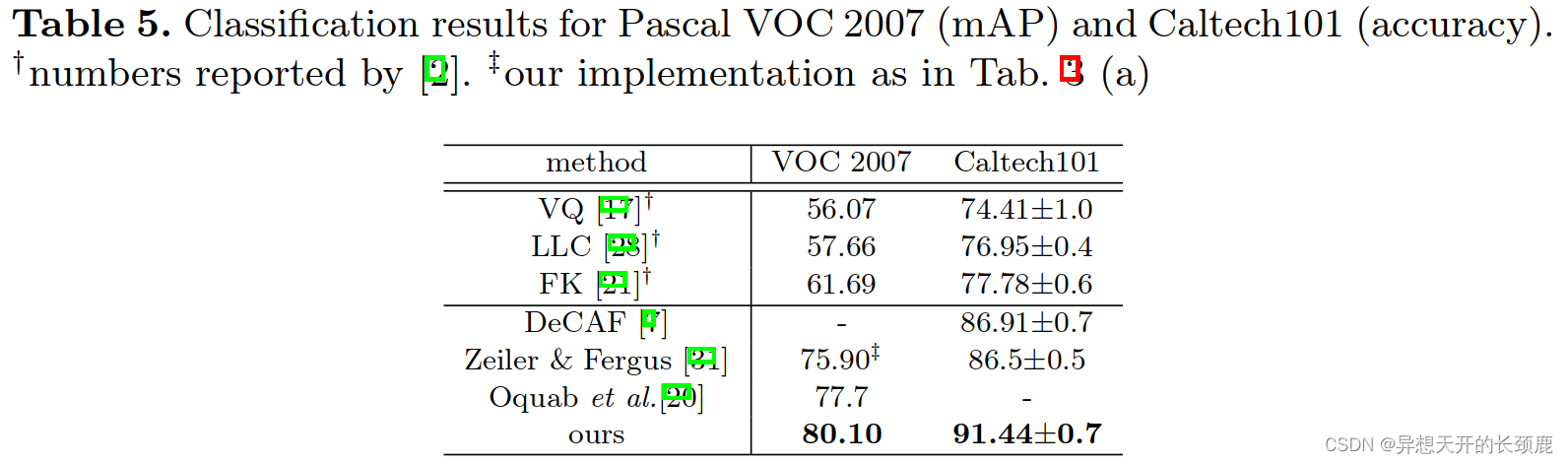
　　Tab. 5 summarizes our results and the comparisons with previous state-ofthe-art methods. Among these methods, VQ [17], LCC [28], and FK [21] are all based on spatial pyramids matching, and [7,31,20] are based on deep networks. Our method outperforms these methods. We note that Oquab et al.[20] achieves 77.7% with 500 views per image, whereas we achieve 80.10% with a single full-image view. Our result may be further improved if data argumentation, multi-view testing, or network fine-tuning is used.
　　表5总结了我们的结果以及与以前的先进方法的比较。在这些方法中，VQ[17]、LCC[28]和FK[21]都是基于空间金字塔匹配，而[7,31,20]是基于深度网络的。我们的方法优于这些方法。我们注意到Oquab等人[20]在每张图片有500个视图的情况下达到了77.7%，而我们在单一的全图视图下达到了80.10%。如果使用数据论证、多视图测试或网络微调，我们的结果可能会进一步提高。

3.3 Experiments on Caltech101（Caltech101实验）

Caltech101 [9] contains 9,144 images in 102 categories (one background). We randomly sample 30 images/category for training and up to 50 images/category for testing. We repeat 10 random splits and average the accuracy.
　　Caltech101[9]包含102个类别（一个背景）的9144张图像。我们随机抽取30张图片/类别进行训练，最多50张图片/类别进行测试。我们重复10次随机拆分，并对准确性进行平均。

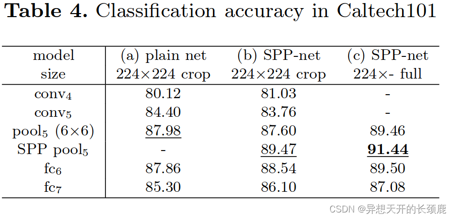
　　Tab. 4 summarizes our results. There are some common observations in the Pascal VOC 2007 and Caltech101 results: SPP-net is better than the plain net (Tab. 4 (b) vs. (a)), and the full-view representation is better than the crop (© vs. (b)). But the results in Caltech101 have some differences with Pascal VOC. The fully-connected layers are less accurate, and the pool5 and SPP layers are better. This is possibly because the object categories in Caltech101 are less related to those in ImageNet, and the deeper layers are more category-specialized. Further, we find that the scale 224 has the best performance among the scales we tested on this dataset. This is mainly because the objects in Caltech101 also occupy large regions of the images, as is the case of ImageNet.
　　表4总结了我们的结果。在Pascal VOC 2007和Caltech101的结果中，有一些共同的看法。SPP网比普通网好（Tab.4 (b) vs. (a)），全视角表现比裁剪好（© vs. (b)）。但是Caltech101的结果与Pascal VOC有一些区别。全连接图层的准确度较低，而pool5和SPP图层则较好。这可能是因为Caltech101中的对象类别与ImageNet中的对象类别关系较小，而较深的层则更具有类别专业性。此外，我们发现，在我们在这个数据集上测试的尺度中，尺度224的性能是最好的。这主要是因为Caltech101中的物体也占据了图像的大区域，就像ImageNet的情况一样。
　　Tab. 5 summarizes our results compared with several previous state-of-the-art methods on Caltech101. Our result (91.44%) exceeds the previous state-of-theart results (86.91%) by a substantial margin (4.5%).

4 SPP-Net for Object Detection（用于目标检测的SPP-Net）

Deep networks have been used for object detection. We briefly review the recent state-of-the-art R-CNN method [12]. R-CNN first extracts about 2,000 candidate windows from each image via selective search [23]. Then the image region in each window is warped to a fixed size (227×227). A pre-trained deep network is used to extract the feature of each window. A binary SVM classifier is then trained on these features for detection. R-CNN generates results of compelling quality and substantially outperforms previous methods (30% relative improvement!). However, because R-CNN repeatedly applies the deep convolutional network to about 2,000 windows per image, it is time-consuming.
　　深度网络已经被用于目标检测。我们简要回顾一下最近最先进的R-CNN方法[12]。R-CNN首先通过选择性搜索[23]从每个图像中提取大约2000个候选窗口。然后，每个窗口中的图像区域被扭曲成一个固定的大小（227×227）。一个预先训练好的深度网络被用来提取每个窗口的特征。然后在这些特征上训练一个二进制SVM分类器进行检测。R-CNN产生的结果具有令人信服的质量，并大大超过了以前的方法（30%的相对改进！）。然而，由于R-CNN将深度卷积网络反复应用于每张图像的大约2000个窗口，因此很耗时。

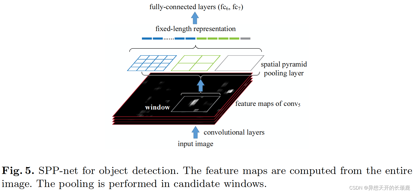
　　Our SPP-net can also be used for object detection. We extract the feature maps from the entire image only once. Then we apply the spatial pyramid pooling on each candidate window of the feature maps to pool a fixed-length representation of this window (see Fig. 5). Because the time-consuming convolutional network is only applied once, our method can run orders of magnitude faster.
　　我们的SPP网络也可用于目标检测。我们只从整个图像中提取一次特征图。然后，我们在特征图的每个候选窗口上应用空间金字塔集合法，以池化这个窗口的固定长度的表示（见图5）。因为耗时的卷积网络只应用一次，所以我们的方法运行速度可以快上几个数量级。
　　Our method extracts window-wise features from regions of the feature maps, while R-CNN extracts directly from image regions. In previous works, the Deformable Part Model (DPM) [10] extracts from windows in HOG [5] feature maps, and Selective Search [23] extracts from windows in encoded SIFT feature maps. The Overfeat detection method [24] also extracts from windows in CNN feature maps, but needs to pre-define the window size. On the contrary, our method enables feature extraction in any windows from CNN feature maps.
　　我们的方法是从特征图的区域中提取窗口特征，而R-CNN则是直接从图像区域中提取。在以前的工作中，可变形部分模型（DPM）[10]从HOG[5]特征图中的窗口提取，而选择性搜索[23]从编码的SIFT特征图中的窗口提取。Overfeat检测方法[24]也是从CNN特征图的窗口中提取，但需要预先定义窗口大小。相反，我们的方法可以从CNN特征图的任何窗口中提取特征。

4.1 Detection Algorithm（检测算法）

We use the “fast” mode of selective search [23] to generate about 2,000 candidate windows per image. Then we resize the image such that min(w, h)=s,and extract the feature maps of conv5 from the entire image. We use our pre-trained model of Tab. 1 (e3) for the time being. In each candidate window, we use a 4-level spatial pyramid (1×1, 2×2, 3×3, 6×6, totally 50 bins) to pool the features. This generates a 12,800-d (256×50) representation for each window. These representations are provided to the fully-connected layers of the network. Then we train a binary linear SVM classifier for each category on these features.
　　我们使用选择性搜索的 "快速 "模式[23]，为每幅图像生成约2,000个候选窗口。然后我们调整图像的大小，使min(w, h)=s，并从整个图像中提取conv5的特征图。我们暂时使用表1(e3)的预训练模型。在每个候选窗口中，我们使用一个4级空间金字塔（1×1，2×2，3×3，6×6，共50个bin）来汇集特征。这就为每个窗口生成了12,800-d（256×50）的表示。这些表征被提供给网络的全连接层。然后我们在这些特征上为每个类别训练一个二元线性SVM分类器。
　　Our implementation of the SVM training follows [23,12]. We use the groundtruth windows to generate the positive samples. The negative samples are those overlapping a positive window by at most 30% . Any negative sample is removed if it overlaps another negative sample by more than 70%. We apply the standard hard negative mining [10] to train the SVM. This step is iterated once. It takes less than 1 hour to train SVMs for all 20 categories. In testing, the classifier is used to score the candidate windows. Then we use non-maximum suppression [10] (threshold of 30%) on the scored windows.
　　我们对SVM训练的实现遵循[23,12]。我们使用真实的窗口来生成正样本。负面样本是那些与正面窗口最多重叠30%的样本。如果任何负样本与另一个负样本重叠超过70%，则被删除。我们应用标准的硬性负面挖掘[10]来训练SVM。这一步骤被反复进行一次。为所有20个类别训练SVM需要不到1小时。在测试中，分类器被用来对候选窗口进行评分。然后我们对得分的窗口使用非最大抑制[10]（阈值为30%）。
　　Our method can be improved by multi-scale feature extraction. We resize the image such that min(w, h)=s ∈S= {480, 576, 688, 864, 1200}, and compute the feature maps of conv5 for each scale. One strategy of combining the features from these scales is to pool them channel-by-channel. But we empirically find that another strategy provides better results. For each candidate window, we choose a single scale s ∈Ssuch that the scaled candidate window has a number of pixels closest to 224×224. Then we only use the feature maps extracted from this scale to compute the feature of this window. If the pre-defined scales are dense enough and the window is approximately square, our method is roughly equivalent to resizing the window to 224×224 and then extracting features from it. Nevertheless, our method only requires computing the feature maps once (at each scale) from the entire image, regardless of the number of candidate windows.
　　我们的方法可以通过多尺度特征提取来改进。我们调整图像的大小，使min(w, h)=s∈S= {480, 576, 688, 864, 1200}，并为每个尺度计算conv5的特征图。结合这些尺度的特征的一个策略是逐个通道汇集它们。但我们根据经验发现，另一种策略可以提供更好的结果。对于每个候选窗口，我们选择一个单一的尺度s∈Ssuch，使该尺度的候选窗口具有最接近224×224的像素数。然后我们只使用从这个尺度中提取的特征图来计算这个窗口的特征。如果预设的尺度足够密集，并且窗口近似于正方形，我们的方法大致相当于将窗口的大小调整为224×224，然后从中提取特征。尽管如此，我们的方法只需要从整个图像中计算一次特征图（在每个尺度上），而不管候选窗口的数量如何。
　　We also fine-tune our pre-trained network, following [12]. Since our features are pooled from the conv5 feature maps from windows of any sizes, for simplicity we only fine-tune the fully-connected layers. In this case, the data layer accepts the fixed-length pooled features after conv5,andthefc6,7 layers and a new 21way (one extra negative category) fc8 layer follow. The fc8 weights are initialized with a Gaussian distribution of σ=0.01. We fix all the learning rates to 1e-4 and then adjust to 1e-5 for all three layers. During fine-tuning, the positive samples are those overlapping with a ground-truth window by [0.5, 1], and the negative samples by [0.1, 0.5). In each mini-batch, 25% of the samples are positive. We train 250k mini-batches using the learning rate 1e-4, and then 50k mini-batches using 1e-5. Because we only fine-tune the fc layers, the training is very fast and takes about 2 hours on the GPU. Also following [12], we use bounding box regression to post-process the prediction windows. The features used for regression are the pooled features from conv5 (as a counterpart of the pool5 features used in [12]). The windows used for the regression training are those overlapping with a ground-truth window by at least 50%.
　　我们还按照文献[12]对我们的预训练网络进行了微调。由于我们的特征是由任何大小的窗口的conv5特征图汇集而成的，为了简单起见，我们只对全连接层进行微调。在这种情况下，数据层接受conv5之后的固定长度的集合特征，fc6,7层和一个新的21路（一个额外的负面类别）fc8层随之而来。fc8的权重是用σ=0.01的高斯分布初始化的。我们将所有的学习率固定为1e-4，然后调整为所有三个层的1e-5。在微调过程中，正样本是那些与真实窗口[0.5, 1]重叠的样本，而负样本是[0.1, 0.5]。在每个小批中，25%的样本是阳性的。我们用1e-4的学习率训练250k个小批，然后用1e-5训练50k个小批。因为我们只对fc层进行微调，所以训练速度非常快，在GPU上大约需要2小时。同样按照[12]，我们使用边界盒回归来对预测窗口进行后处理。用于回归的特征是conv5的集合特征（与[12]中使用的pool5特征相对应）。用于回归训练的窗口是那些与地面实况窗口重叠至少50%的窗口。
　　We will release the code to facilitate reproduction of the results(research.microsoft.com/en-us/um/people/kahe/).
　　我们将发布代码，以促进结果的复制（research.microsoft.com/en-us/um/people/kahe/）。

4.2 Detection Results（检测结果）

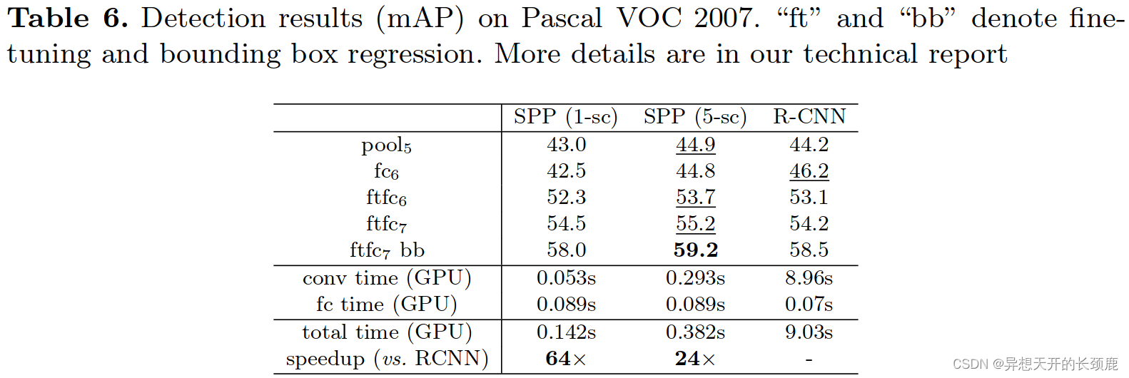
We evaluate our method on the detection task of the Pascal VOC 2007 dataset. Tab. 6 shows our results on various layers, by using 1-scale (s=688) or 5-scale. Using the pool5 layers (in our case the pooled features), our result (44.9%) is comparable with R-CNN’s result (44.2%). But using the non-fine-tuned fc6 layers, our results are inferior. An explanation is that our fc layers are pre-trained using image regions, while in the detection case they are used on the feature map regions. The feature map regions can have strong activations near the window boundaries, while the image regions may not. This difference of usages can be addressed by fine-tuning. Using the fine-tuned fc layers (ftfc6,7), our results are comparable with or slightly better than the fine-tuned results of R-CNN. After bounding box regression, our 5-scale result (59.2%) is 0.7% better than R-CNN (58.5%), and our 1-scale result (58.0%) is 0.5% worse. In Tab. 7, we show the results for each category. Our method outperforms R-CNN in 11 categories, and has comparable numbers in two more categories.
　　我们在Pascal VOC 2007数据集的检测任务上评估了我们的方法。表6显示了我们在不同层的结果，通过使用1种尺度（s=688）或5种尺度。使用pool5层（在我们的例子中是集合特征），我们的结果（44.9%）与R-CNN的结果（44.2%）相当。但是使用非微调的fc6层，我们的结果要差一些。一个解释是，我们的fc层是使用图像区域进行预训练的，而在检测情况下，它们被用于特征图区域。特征图区域在窗口边界附近可能有很强的激活，而图像区域可能没有。这种使用上的差异可以通过微调来解决。使用微调的fc层（ftfc6,7），我们的结果与R-CNN的微调结果相当或略好。在边界盒回归后，我们的5尺度结果（59.2%）比R-CNN（58.5%）好0.7%，而我们的1尺度结果（58.0%）则差0.5%。在表7中，我们显示了每个类别的结果。我们的方法在11个类别中优于R-CNN，并在另外两个类别中具有相当的数字。


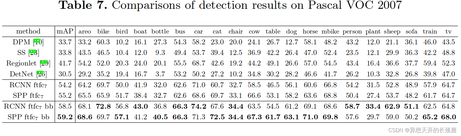
　　In Tab. 7, Selective Search (SS) [23] applies spatial pyramid matching on SIFT feature maps. DPM [10] and Regionlet [29] are based on HOG features [5]. Regionlet improves to 46.1% [33] by combining various features including conv5. DetectorNet [26] trains a deep network that outputs pixel-wise object masks. This method only needs to apply the deep network once to the entire image, as is the case for our method. But this method has lower mAP (30.5%).
　　在表7中，选择性搜索（SS）[23]在SIFT特征图上应用空间金字塔匹配。DPM[10]和Regionlet[29]是基于HOG特征[5]的。Regionlet通过结合包括conv5在内的各种特征提高到46.1%[33]。DetectorNet[26]训练了一个深度网络，输出像素级的物体掩码。这个方法只需要对整个图像应用一次深度网络，我们的方法也是如此。但是这个方法的mAP较低（30.5%）。

4.3 Complexity and Running Time（复杂度和运行时间）

Despite having comparable accuracy, our method is much faster than R-CNN. The complexity of the convolutional feature computation in R-CNN is O(n · 2272) with the window number n (∼2000). This complexity of our method is O(r · s2)atascales,wherer is the aspect ratio. Assume r is about 4/3. In the single-scale version when s = 688, this complexity is about 1/160 of R-CNN’s; in the 5-scale version, this complexity is about 1/24 of R-CNN’s. In Tab. 6, we compare the experimental running time of the convolutional feature computation. The implementation of R-CNN is from the code published by the authors implemented in Caffe [7]. For fair comparison, we also implement our feature computation in Caffe. In Tab. 6 we evaluate the average time of 100 random VOC images using GPU. R-CNN takes 8.96s per image, while our 1-scale version takes only 0.053s per image. So ours is 170× faster than R-CNN. Our 5-scale version takes 0.293s per image, so is 30× faster than R-CNN.
　　尽管有相当的准确性，我们的方法比R-CNN快得多。R-CNN中卷积特征计算的复杂度是O(n - 2272)，窗口数为n(∼2000)。我们的方法的复杂度是O(r - s2)级，其中r是长宽比。假设r约为4/3。在s=688的单尺度版本中，这一复杂度大约是R-CNN的1/160；在5尺度版本中，这一复杂度大约是R-CNN的1/24。在表6中，我们比较了卷积特征计算的实验运行时间。R-CNN的实现来自作者发表的在Caffe[7]中实现的代码。为了公平比较，我们也在Caffe中实现了我们的特征计算。在表6中，我们评估了使用GPU计算100张随机VOC图像的平均时间。R-CNN每幅图像需要8.96秒，而我们的1尺度版本每幅图像只需要0.053秒。所以我们的版本比R-CNN快170倍。我们的5尺度版本每幅图像需要0.293秒，所以比R-CNN快30倍。
　　Our convolutional feature computation is so fast that the computational time of fc layers takes a considerable portion. Tab. 6 shows that the GPU time of computing the 4,096-d fc7 features (from the conv5 feature maps) is 0.089s per image. Considering both convolutional and fully-connected features, our 1-scale version is 64× faster than R-CNN and is just 0.5% inferior in mAP; our 5-scale version is 24× faster and has better results. The overhead of the fc computation can be significantly reduced if smaller fc layers are used, e.g., 1,024-d.
　　我们的卷积特征计算是如此之快，以至于fc层的计算时间占了相当大的比重。表6显示，计算4,096-d fc7特征（来自conv5特征图）的GPU时间为每张图像0.089s。考虑到卷积和全连接的特征，我们的1尺度版本比R-CNN快64倍，在mAP中仅差0.5%；我们的5尺度版本快24倍，并且有更好的结果。如果使用较小的fc层，例如1,024-d，fc计算的开销可以大大减少。
　　We do not consider the window proposal time in the above comparison. The selective search window proposal [23] takes about 1-2 seconds per image on the CPU. There are recent works (e.g., [3]) on reducing window proposal time to milliseconds. We will evaluate this and expect a fast entire system.
　　在上述比较中，我们不考虑窗口提议的时间。选择性搜索窗口建议[23]在CPU上每幅图像需要大约1-2秒。最近有一些工作（例如，[3]）是关于将窗口提议时间减少到几毫秒。我们将对此进行评估，并期待整个系统的快速发展。

4.4 Model Combination for Detection（检测的模型组合）

Model combination is an important strategy for boosting CNN-based classification accuracy [16]. Next we propose a simple model combination method for detection. We pre-train another network in ImageNet, using the same structure but different random initializations. Then we repeat the above detection algorithm. Tab. 8 (SPP-net (2)) shows the results of this network. Its mAP is comparable with the first network (59.1% vs. 59.2%), and outperforms the first network in 11 categories. Given the two models, we first use either model to score all candidate windows on the test image. Then we perform non-maximum suppression on the union of the two sets of candidate windows (with their scores). A more confident window given by one method can suppress those less confident given by the other method. After combination, the mAP is boosted to 60.9% (Tab. 8). In 17 out of all 20 categories the combination performs better than either individual model. This indicates that the two models are complementary.
　　模型组合是提升基于CNN分类准确性的重要策略[16]。接下来我们提出一个简单的模型组合检测方法。我们在ImageNet中预先训练另一个网络，使用相同的结构但不同的随机初始化。然后我们重复上述的检测算法。表8. 8（SPP-net (2)）显示了这个网络的结果。它的mAP与第一个网络相当（59.1% vs. 59.2%），并在11个类别中优于第一个网络。考虑到这两个模型，我们首先使用任一模型对测试图像上的所有候选窗口进行评分。然后，我们对两组候选窗口的联合体（连同它们的分数）进行非最大限度的压制。一种方法给出的更有信心的窗口可以压制另一种方法给出的信心不足的窗口。组合之后，mAP被提升到60.9%（表8）。在所有20个类别中的17个中，组合的表现比任何一个单独的模型都好。这表明这两个模型是互补的。

5 Conclusion（结论）

Image scales and sizes are important in visual recognition, but received little consideration in the context of deep networks. We have suggested a solution to train a deep network with an SPP layer. The resulting SPP-net shows outstanding accuracy in classification/detection tasks and greatly accelerates DNN-based detection. Our studies also show that many time-proven techniques/insights in computer vision can still play important roles in deep-networks-based recognition.
　　图像的尺度和尺寸在视觉识别中很重要，但在深度网络的背景下很少得到考虑。我们提出了一个解决方案，用SPP层训练一个深度网络。由此产生的SPP-网络在分类/检测任务中显示出杰出的准确性，并大大加速了基于DNN的检测。我们的研究还表明，计算机视觉中许多经过时间验证的技术/见解仍然可以在基于深度网络的识别中发挥重要作用。