matplotlib画图

matplotlib画图

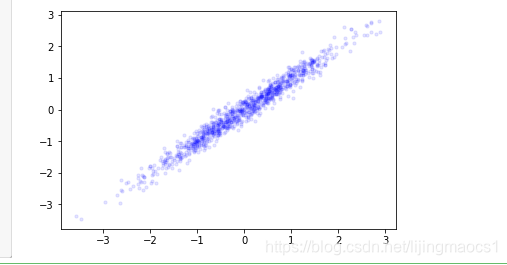
散点图

## s:点大小
## c:颜色
## marker:点的样式
## alpha:透明度

x = np.random.randn(1000)
y=x+np.random.randn(1000)*0.2
plt.scatter(x,y,s=10,c='b',alpha=0.1)
plt.show()

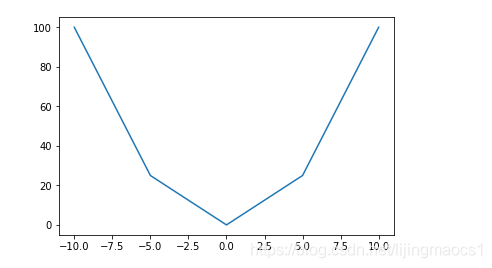
折线图

x=np.linspace(-10,10,5)
y=x**2
plt.plot(x,y)

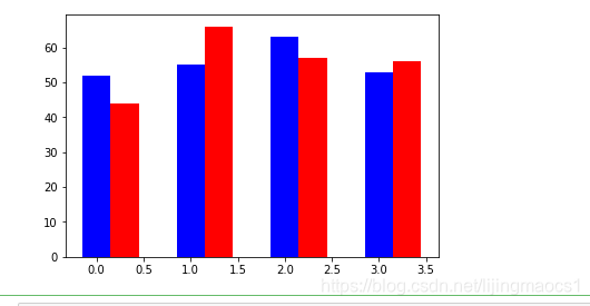
柱状图

sales_bj = [52,55,63,53]
sales_sh = [44,66,57,56]
bar_with = 0.3
index = np.arange(4)
plt.bar(index,sales_bj,bar_with,color='b')
plt.bar(index+bar_with,sales_sh,bar_with,color='r')

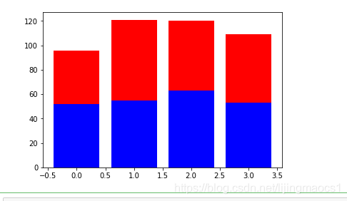
plt.bar(index,sales_bj,color='b')
plt.bar(index,sales_sh,color='r',bottom=sales_bj)

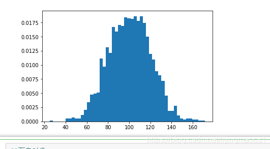
直方图

mu =100
sigma = 20
x=mu+sigma*np.random.randn(2000)
plt.hist(x,bins=50,normed=True)

面向对象

x = np.arange(0,10,1)
y = np.random.randn(len(x))
#生成一个figure对象#
fig = plt.figure()
#添加子图#
ax1 = fig.add_subplot(2,2,1)
ax2 = fig.add_subplot(2,2,2)

ax1.plot(x,y)
ax2.plot(x,-y)

plt.show()

#生成2个figur()，2个图
fig1 = plt.figure()
fig2 = plt.figure()

#生成网格#
plt.grid(True)
#取消网格#
plt.grid()
#设置网格属性#
plt.grid(color='r',linewith='2',linestyle='-')

#面向对象方式生成网格#
ax1.grid(color='r')

##图例
plt.plot(x,x*2,lable='Normal')
plt.plot(x,x*3,lable='Fast')
plt.plot(x,x*4,lable='Faster')
#显示图例#
plt.legend(loc=1) #loc 位置参数 0,1,2,3,4//0=best
plt.legend(ncol=3) #ncol 列数

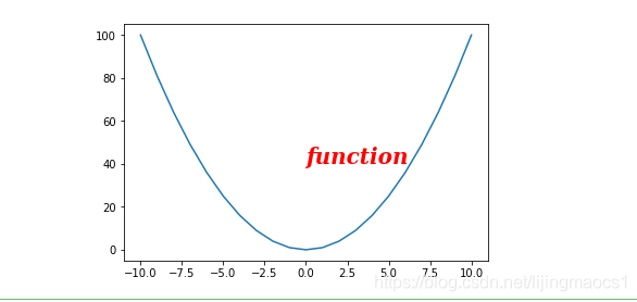
注释

x=np.arange(-10,11)
y=x*x

plt.text(0,40,'function',family='serif',color='r',size=20,style='italic',weight='black')
plt.plot(x,y)

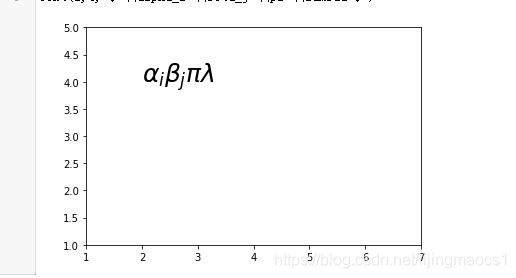
怎么写数学公式

fig= plt.figure()
ax = fig.add_subplot(1,1,1)
ax.set_xlim([1,7])
ax.set_ylim([1,5])
ax.text(2,4,r"$ \alpha_i \beta_j \pi \lambda $",size=25)

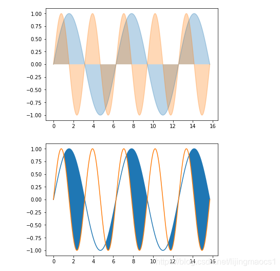
区域填充

x=np.linspace(0,5*np.pi,1000)
y1 = np.sin(x)
y2 = np.sin(2*x)
plt.plot(x,y1,alpha=0.3)
plt.plot(x,y2,alpha=0.3)
#plt.grid()
plt.fill(x,y1,alpha=0.3)
plt.fill(x,y2,alpha=0.3)
##方法2
fig = plt.figure()
ax = fig.add_subplot(1,1,1)
ax.plot(x,y1)
ax.plot(x,y2)
ax.fill_between(x,y1,y2,where=y1>=y2)

美化,风格选择

plt.style.available
plt.style.ues('classic')

极坐标

r = np.arange(1,6)
theta = [0,np.pi/2,np.pi,3*np.pi/2,2*np.pi]
ax = plt.subplot(111,projection='polar')
ax.plot(r,theta)
plt.show()