河北高校邀请赛——二手车交易价格预测-Task2 EDA

本文链接：https://blog.csdn.net/liu_dongd/article/details/115893003

EDA

import warnings
warnings.filterwarnings('ignore')
import pandas as pd
import numpy as np
import matplotlib.pyplot as plt
import seaborn as sns
from sklearn.model_selection import KFold
from lightgbm.sklearn import LGBMRegressor
from sklearn.metrics import mean_squared_error, mean_absolute_error
import time

#导入数据
Train_data = pd.read_csv('car_train_0110.csv', sep=' ')
Test_data = pd.read_csv('car_testA_0110.csv', sep=' ')

# 合并方便后面的操作
df = pd.concat([Train_data, Test_data], ignore_index=True)

# 看下数据的情况，前后各5行
Train_data.head().append(Train_data.tail())

	SaleID	name	regDate	model	brand	bodyType	fuelType	gearbox	power	kilometer	...	v_14	v_15	v_16	v_17	v_18	v_19	v_20	v_21	v_22	v_23
0	134890	734	20160002	13.0	9	NaN	0.0	1.0	0	15.0	...	0.092139	0.000000	18.763832	-1.512063	-1.008718	-12.100623	-0.947052	9.077297	0.581214	3.945923
1	306648	196973	20080307	72.0	9	7.0	5.0	1.0	173	15.0	...	0.001070	0.122335	-5.685612	-0.489963	-2.223693	-0.226865	-0.658246	-3.949621	4.593618	-1.145653
2	340675	25347	20020312	18.0	12	3.0	0.0	1.0	50	12.5	...	0.064410	0.003345	-3.295700	1.816499	3.554439	-0.683675	0.971495	2.625318	-0.851922	-1.246135
3	57332	5382	20000611	38.0	8	7.0	0.0	1.0	54	15.0	...	0.069231	0.000000	-3.405521	1.497826	4.782636	0.039101	1.227646	3.040629	-0.801854	-1.251894
4	265235	173174	20030109	87.0	0	5.0	5.0	1.0	131	3.0	...	0.000099	0.001655	-4.475429	0.124138	1.364567	-0.319848	-1.131568	-3.303424	-1.998466	-1.279368
249995	10556	9332	20170003	13.0	9	NaN	NaN	1.0	58	15.0	...	0.079119	0.001447	11.782508	20.402576	-2.722772	0.462388	-4.429385	7.883413	0.698405	-1.082013
249996	146710	102110	20030511	29.0	17	3.0	0.0	0.0	61	15.0	...	0.000000	0.002342	-2.988272	1.500532	3.502201	-0.761715	-2.484556	-2.532968	-0.940266	-1.106426
249997	116066	82802	20130312	124.0	16	6.0	0.0	1.0	122	3.0	...	0.003358	0.100760	-6.939560	-1.144959	-5.337949	0.896026	-0.592565	-3.872725	2.135984	3.807554
249998	90082	65971	20121212	111.0	4	7.0	5.0	0.0	184	9.0	...	0.002974	0.008251	-7.222167	-1.383696	-5.402794	-0.409451	-1.891556	-3.104789	-3.777374	3.186218
249999	76453	56954	20051111	13.0	9	3.0	0.0	1.0	58	12.5	...	0.000000	0.009071	10.491312	-11.270043	-0.272595	-0.026478	-2.168249	-0.980042	-0.955164	-1.169593

10 rows × 40 columns

Test_data.head().append(Train_data.tail())

	SaleID	name	regDate	model	brand	bodyType	fuelType	gearbox	power	kilometer	...	v_15	v_16	v_17	v_18	v_19	v_20	v_21	v_22	v_23	price
0	720326	505	20060505	19.0	13	7.0	0.0	1.0	90	8.0	...	0.105382	-5.998993	0.147048	-1.902847	0.348990	2.324961	3.343910	4.048742	-1.431822	NaN
1	714316	1836	20010301	5.0	5	3.0	4.0	1.0	75	15.0	...	0.000000	-3.287221	2.081317	2.937052	-0.123018	1.202395	3.570743	-1.180587	-1.348598	NaN
2	704693	212291	20170610	6.0	18	NaN	5.0	0.0	150	15.0	...	0.000000	4.368218	8.252188	-4.136109	-13.334970	-4.444620	-0.706978	-1.720218	3.569112	NaN
3	624972	1345	19820005	215.0	32	7.0	0.0	1.0	0	6.0	...	0.100883	-2.537486	0.513955	4.414962	0.357685	2.700732	5.323602	6.085956	-0.900585	NaN
4	669753	1428	20060205	30.0	4	7.0	5.0	1.0	122	15.0	...	0.002509	-6.197633	-0.191814	-1.224360	-0.326985	2.254931	4.183037	-2.574004	0.014203	NaN
249995	10556	9332	20170003	13.0	9	NaN	NaN	1.0	58	15.0	...	0.001447	11.782508	20.402576	-2.722772	0.462388	-4.429385	7.883413	0.698405	-1.082013	1200.0
249996	146710	102110	20030511	29.0	17	3.0	0.0	0.0	61	15.0	...	0.002342	-2.988272	1.500532	3.502201	-0.761715	-2.484556	-2.532968	-0.940266	-1.106426	1200.0
249997	116066	82802	20130312	124.0	16	6.0	0.0	1.0	122	3.0	...	0.100760	-6.939560	-1.144959	-5.337949	0.896026	-0.592565	-3.872725	2.135984	3.807554	16500.0
249998	90082	65971	20121212	111.0	4	7.0	5.0	0.0	184	9.0	...	0.008251	-7.222167	-1.383696	-5.402794	-0.409451	-1.891556	-3.104789	-3.777374	3.186218	31950.0
249999	76453	56954	20051111	13.0	9	3.0	0.0	1.0	58	12.5	...	0.009071	10.491312	-11.270043	-0.272595	-0.026478	-2.168249	-0.980042	-0.955164	-1.169593	1990.0

10 rows × 40 columns

# 查看总体情况，个数，平均值，方差等
Train_data.describe()

	SaleID	name	regDate	model	brand	bodyType	fuelType	gearbox	power	kilometer	...	v_14	v_15	v_16	v_17	v_18	v_19	v_20	v_21	v_22	v_23
count	250000.000000	250000.000000	2.500000e+05	250000.000000	250000.000000	224620.000000	227510.000000	236487.000000	250000.000000	250000.000000	...	250000.000000	250000.000000	250000.000000	250000.000000	250000.000000	250000.000000	250000.000000	250000.000000	250000.000000	250000.000000
mean	185351.790768	83153.362172	2.003401e+07	44.911480	7.785236	4.563271	1.665008	0.780783	115.528412	12.577418	...	0.032489	0.030408	0.014725	0.000915	0.006273	0.006604	-0.001374	0.000609	-0.004025	0.001834
std	107121.188763	72540.799964	7.770250e+04	50.640081	7.694010	1.912515	2.339646	0.413717	196.141828	3.990632	...	0.038792	0.049333	8.779163	5.771081	4.880981	4.124722	3.803626	3.555353	2.864713	2.323680
min	1.000000	0.000000	1.910000e+07	0.000000	0.000000	0.000000	0.000000	0.000000	0.000000	0.500000	...	0.000000	0.000000	-10.412444	-15.538236	-21.009214	-13.989955	-9.599285	-11.181255	-7.671327	-2.350888
25%	92501.750000	14500.000000	1.999061e+07	6.000000	1.000000	3.000000	0.000000	1.000000	70.000000	12.500000	...	0.000129	0.000000	-5.552269	-0.901181	-3.150385	-0.478173	-1.727237	-3.067073	-2.092178	-1.402804
50%	185264.500000	65314.500000	2.003111e+07	27.000000	6.000000	4.000000	0.000000	1.000000	105.000000	15.000000	...	0.001961	0.002567	-3.821770	0.223181	-0.058502	0.038427	-0.995044	-0.880587	-1.199807	-1.145588
75%	278128.500000	143761.250000	2.008081e+07	70.000000	11.000000	7.000000	5.000000	1.000000	150.000000	15.000000	...	0.075672	0.056568	3.599747	1.263737	2.800475	0.569198	1.563382	3.269987	2.737614	0.044865
max	370946.000000	233044.000000	2.019121e+07	250.000000	39.000000	7.000000	6.000000	1.000000	20000.000000	15.000000	...	0.130785	0.184340	36.756878	26.134561	23.055660	16.576027	20.324572	14.039422	8.764597	8.574730

8 rows × 40 columns

Test_data.describe()

	SaleID	name	regDate	model	brand	bodyType	fuelType	gearbox	power	kilometer	...	v_14	v_15	v_16	v_17	v_18	v_19	v_20	v_21	v_22	v_23
count	50000.000000	50000.000000	5.000000e+04	50000.000000	50000.000000	44890.000000	45598.000000	47287.000000	50000.000000	50000.000000	...	50000.000000	50000.000000	50000.000000	50000.000000	50000.000000	50000.000000	50000.000000	50000.000000	50000.000000	50000.000000
mean	556029.053380	82878.251420	2.003441e+07	44.922840	7.779420	4.556226	1.681192	0.781081	114.116060	12.555210	...	0.032570	0.030773	-0.024819	0.007051	-0.008488	-0.030104	0.014609	-0.003353	0.013125	-0.011936
std	106952.402565	72292.076936	7.788055e+04	50.576255	7.661667	1.908291	2.344829	0.413518	177.274154	4.034901	...	0.038779	0.049521	8.759663	5.784299	4.825261	4.100561	3.812667	3.548944	2.866774	2.316144
min	370951.000000	0.000000	1.910000e+07	0.000000	0.000000	0.000000	0.000000	0.000000	0.000000	0.500000	...	0.000000	0.000000	-10.196998	-15.167961	-21.925773	-13.682825	-9.282567	-11.117367	-6.365723	-2.394516
25%	463258.500000	14121.250000	1.999061e+07	6.000000	1.000000	3.000000	0.000000	1.000000	69.000000	12.500000	...	0.000135	0.000000	-5.575131	-0.891030	-3.105073	-0.481952	-1.697763	-3.069575	-2.089326	-1.402958
50%	556296.000000	65359.000000	2.003111e+07	27.000000	6.000000	4.000000	0.000000	1.000000	105.000000	15.000000	...	0.001949	0.002593	-3.837572	0.221379	-0.081836	0.039376	-0.971210	-0.877377	-1.192502	-1.146398
75%	648862.250000	143083.750000	2.008091e+07	70.000000	11.000000	7.000000	5.000000	1.000000	150.000000	15.000000	...	0.075826	0.062063	3.531269	1.257687	2.784538	0.560046	1.572508	3.276918	2.772742	-0.010769
max	741887.000000	233028.000000	2.019040e+07	248.000000	39.000000	7.000000	6.000000	1.000000	17700.000000	15.000000	...	0.135900	0.180091	36.364986	26.043572	22.598441	16.333051	20.273633	11.691851	7.970303	8.749647

8 rows × 39 columns

Train_data.shape

(250000, 40)

Test_data.shape

(50000, 39)

#查看数据信息
df.info()
#查看缺失值
df.isnull().sum()

<class 'pandas.core.frame.DataFrame'>
RangeIndex: 300000 entries, 0 to 299999
Data columns (total 40 columns):
 #   Column             Non-Null Count   Dtype  
---  ------             --------------   -----  
 0   SaleID             300000 non-null  int64  
 1   name               300000 non-null  int64  
 2   regDate            300000 non-null  int64  
 3   model              300000 non-null  float64
 4   brand              300000 non-null  int64  
 5   bodyType           269510 non-null  float64
 6   fuelType           273108 non-null  float64
 7   gearbox            283774 non-null  float64
 8   power              300000 non-null  int64  
 9   kilometer          300000 non-null  float64
 10  notRepairedDamage  241836 non-null  float64
 11  regionCode         300000 non-null  int64  
 12  seller             300000 non-null  int64  
 13  offerType          300000 non-null  int64  
 14  creatDate          300000 non-null  int64  
 15  price              250000 non-null  float64
 16  v_0                300000 non-null  float64
 17  v_1                300000 non-null  float64
 18  v_2                300000 non-null  float64
 19  v_3                300000 non-null  float64
 20  v_4                300000 non-null  float64
 21  v_5                300000 non-null  float64
 22  v_6                300000 non-null  float64
 23  v_7                300000 non-null  float64
 24  v_8                300000 non-null  float64
 25  v_9                300000 non-null  float64
 26  v_10               300000 non-null  float64
 27  v_11               300000 non-null  float64
 28  v_12               300000 non-null  float64
 29  v_13               300000 non-null  float64
 30  v_14               300000 non-null  float64
 31  v_15               300000 non-null  float64
 32  v_16               300000 non-null  float64
 33  v_17               300000 non-null  float64
 34  v_18               300000 non-null  float64
 35  v_19               300000 non-null  float64
 36  v_20               300000 non-null  float64
 37  v_21               300000 non-null  float64
 38  v_22               300000 non-null  float64
 39  v_23               300000 non-null  float64
dtypes: float64(31), int64(9)
memory usage: 91.6 MB





SaleID                   0
name                     0
regDate                  0
model                    0
brand                    0
bodyType             30490
fuelType             26892
gearbox              16226
power                    0
kilometer                0
notRepairedDamage    58164
regionCode               0
seller                   0
offerType                0
creatDate                0
price                50000
v_0                      0
v_1                      0
v_2                      0
v_3                      0
v_4                      0
v_5                      0
v_6                      0
v_7                      0
v_8                      0
v_9                      0
v_10                     0
v_11                     0
v_12                     0
v_13                     0
v_14                     0
v_15                     0
v_16                     0
v_17                     0
v_18                     0
v_19                     0
v_20                     0
v_21                     0
v_22                     0
v_23                     0
dtype: int64

# nan可视化
missing = Train_data.isnull().sum()
missing = missing[missing > 0]
missing.sort_values(inplace=True)
missing.plot.bar()

<AxesSubplot:>




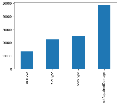
![在这里插入图片描述](https://img-blog.csdnimg.cn/20210420093945341.png?x-oss-process=image/watermark,type_ZmFuZ3poZW5naGVpdGk,shadow_10,text_aHR0cHM6Ly9ibG9nLmNzZG4ubmV0L2xpdV9kb25nZA==,size_16,color_FFFFFF,t_70#pic_center)

字段表如下，可以从上述输出看到，bodyType,fuelType,gearbox,otRepairedDamage这几个项存在着缺失值,缺失值的个数均在10000个以上，缺失值的个数较多，在后续处理中需要考虑是进一步填充（众数，中位数,随机森林），还是删掉。

Field	Description
SaleID	交易ID，唯一编码
name	汽车交易名称，已脱敏
regDate	汽车注册日期，例如20160101，2016年01月01日
model	车型编码，已脱敏
brand	汽车品牌，已脱敏
bodyType	车身类型：豪华轿车：0，微型车：1，厢型车：2，大巴车：3，敞篷车：4，双门汽车：5，商务车：6，搅拌车：7
fuelType	燃油类型：汽油：0，柴油：1，液化石油气：2，天然气：3，混合动力：4，其他：5，电动：6
gearbox	变速箱：手动：0，自动：1
power	发动机功率：范围 [ 0, 600 ]
kilometer	汽车已行驶公里，单位万km
notRepairedDamage	汽车有尚未修复的损坏：是：0，否：1
regionCode	地区编码，已脱敏
seller	销售方：个体：0，非个体：1
offerType	报价类型：提供：0，请求：1
creatDate	汽车上线时间，即开始售卖时间
price	二手车交易价格（预测目标）
v系列特征	匿名特征，包含v0-23在内24个匿名特征

# 查看非匿名类别特征nunique分布
cat_fea = ['name', 'regDate', 'model', 'brand', 'bodyType', 'fuelType',
           'gearbox', 'kilometer', 'notRepairedDamage', 'regionCode',
           'seller', 'offerType', 'creatDate', 'power', 'price']
for fea in cat_fea:
    print(fea + "的特征分布如下：")
    print("{}特征有个{}不同的值".format(fea,df[fea].nunique()))
    print(df[fea].value_counts())

name的特征分布如下：
name特征有个193159不同的值
73        527
451       526
1791      497
821       480
243       423
         ... 
224566      1
204088      1
212284      1
210237      1
84137       1
Name: name, Length: 193159, dtype: int64
regDate的特征分布如下：
regDate特征有个7797不同的值
20000010    356
20000007    353
20000002    351
20000001    336
20000006    328
           ... 
19700511      1
19780406      1
19610603      1
19840603      1
19640202      1
Name: regDate, Length: 7797, dtype: int64
model的特征分布如下：
model特征有个251不同的值
0.0      24260
6.0      21237
4.0      16639
1.0      16440
12.0     10586
         ...  
247.0        7
226.0        7
243.0        5
249.0        4
250.0        1
Name: model, Length: 251, dtype: int64
brand的特征分布如下：
brand特征有个40不同的值
0     64396
4     32573
11    32318
10    28509
1     26534
6     20698
9     14618
5      8877
15     7825
12     5633
7      4621
3      4567
17     4275
13     4181
8      4040
28     3806
19     3095
18     2938
16     2732
22     2694
23     2485
14     2308
24     2068
25     1908
20     1903
27     1657
29     1495
34     1169
30      737
2       671
21      643
31      627
38      608
35      491
32      476
36      450
33      429
37      385
26      379
39      181
Name: brand, dtype: int64
bodyType的特征分布如下：
bodyType特征有个8不同的值
7.0    77319
3.0    64666
4.0    54789
5.0    24518
6.0    18369
2.0    15239
1.0    11862
0.0     2748
Name: bodyType, dtype: int64
fuelType的特征分布如下：
fuelType特征有个7不同的值
0.0    180709
5.0     87139
4.0      4331
3.0       458
2.0       226
1.0       170
6.0        75
Name: fuelType, dtype: int64
gearbox的特征分布如下：
gearbox特征有个2不同的值
1.0    221580
0.0     62194
Name: gearbox, dtype: int64
kilometer的特征分布如下：
kilometer特征有个13不同的值
15.0    194697
12.5     30744
10.0     12840
9.0      10101
8.0       8939
7.0       7905
6.0       7016
5.0       6150
0.5       5588
4.0       5079
3.0       4877
2.0       4553
1.0       1511
Name: kilometer, dtype: int64
notRepairedDamage的特征分布如下：
notRepairedDamage特征有个2不同的值
1.0    212477
0.0     29359
Name: notRepairedDamage, dtype: int64
regionCode的特征分布如下：
regionCode特征有个8122不同的值
487     672
868     517
149     280
539     273
32      262
       ... 
8145      1
8088      1
7989      1
7523      1
6712      1
Name: regionCode, Length: 8122, dtype: int64
seller的特征分布如下：
seller特征有个2不同的值
1    299999
0         1
Name: seller, dtype: int64
offerType的特征分布如下：
offerType特征有个2不同的值
0    299990
1        10
Name: offerType, dtype: int64
creatDate的特征分布如下：
creatDate特征有个110不同的值
20160403    11671
20160404    11387
20160320    10934
20160312    10776
20160321    10744
            ...  
20151123        1
20160114        1
20151014        1
20140310        1
20160115        1
Name: creatDate, Length: 110, dtype: int64
power的特征分布如下：
power特征有个738不同的值
0       32800
75      19385
60      12911
150     12430
140     11012
        ...  
312         1
417         1
672         1
1082        1
1653        1
Name: power, Length: 738, dtype: int64
price的特征分布如下：
price特征有个4585不同的值
0.0        7312
500.0      3815
1500.0     3587
1000.0     3149
1200.0     3071
           ... 
11140.0       1
6165.0        1
5827.0        1
89700.0       1
706.0         1
Name: price, Length: 4585, dtype: int64

#类别特征取值较少的，画出直方图,
#'seller,offerType'数值分布极不平衡
plt.figure()
plt.figure(figsize=(16, 6))
i = 1
for fea in cat_fea:
    if df[fea].nunique()<50:
        plt.subplot(2, 4, i)
        i += 1
        v = df[fea].value_counts()
        fig = sns.barplot(x=v.index, y=v.values)
        for item in fig.get_xticklabels():
            item.set_rotation(90)
        plt.title(fea)
plt.tight_layout()
plt.show()

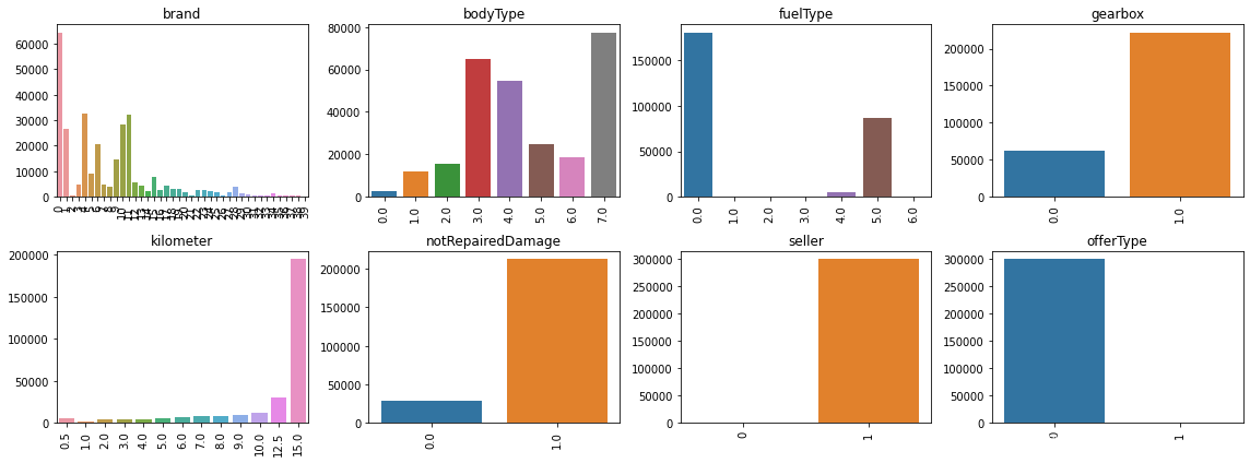
![在这里插入图片描述](https://img-blog.csdnimg.cn/20210420094014831.png?x-oss-process=image/watermark,type_ZmFuZ3poZW5naGVpdGk,shadow_10,text_aHR0cHM6Ly9ibG9nLmNzZG4ubmV0L2xpdV9kb25nZA==,size_16,color_FFFFFF,t_70#pic_center)

seller特征有个2不同的值分别为1（299999）和0（1）这种情况下可以考虑把该特征去掉。
offerType特征有个2不同的值分别为1（10）和0（299990）这种情况下可以考虑把该特征去掉。

# 绘制price的图像
plt.figure()
plt.figure(figsize=(10, 3))
plt.subplot(1, 2,1)
sns.distplot(Train_data['price'])
plt.subplot(1,2,2)
Train_data['price'].plot.box()
plt.tight_layout()

在这里插入图片描述

price呈现长尾分布，后续需要处理，对数变换

#'price'转化后的分布
plt.figure()
sns.distplot(np.log1p(Train_data['price']))

在这里插入图片描述

转换后的price并不是一个标准的正态分布的形状，可以看到有两个峰，左边峰值较小，可以考虑进行处理。

# 处理price,去掉为0的行
df.drop(df[df['price'] == 0].index, inplace=True)
plt.figure()
sns.distplot(np.log1p(df['price']))

在这里插入图片描述

#探索匿名特征的数值特征分布
num_fea = ['v_0', 'v_1', 'v_2', 'v_3',
       'v_4', 'v_5', 'v_6', 'v_7', 'v_8', 'v_9', 'v_10', 'v_11', 'v_12',
       'v_13', 'v_14', 'v_15', 'v_16', 'v_17', 'v_18', 'v_19', 'v_20', 'v_21',
       'v_22', 'v_23']

f = pd.melt(Train_data, value_vars=num_fea)
g = sns.FacetGrid(f, col="variable",  col_wrap=3, sharex=False, sharey=False)
g = g.map(sns.distplot, "value")

在这里插入图片描述

#选取类别特征取值较少的，观察它们与价格的均值分布
plt.figure()
plt.figure(figsize=(20, 18))
i = 1
for f in cat_fea:
    if df[f].nunique() <= 50:
        plt.subplot(5, 3, i)
        i += 1
        v = df[~df['price'].isnull()].groupby(f,as_index=False)['price'].agg({f + '_price_mean': 'mean'}).reset_index()
        fig = sns.barplot(x=f, y=f + '_price_mean', data=v)
        for item in fig.get_xticklabels():
            item.set_rotation(90)
plt.tight_layout()
plt.show()

在这里插入图片描述

# 相关性分析
num_fea.append('price')
corr1 = abs(df[df['price'].notnull()][num_fea].corr())
plt.figure(figsize=(10, 10))
sns.heatmap(corr1, linewidths=0.1, cmap=sns.cm.rocket_r)

在这里插入图片描述