ccc-sklearn-8-SVM（2）

1.SVM重要参数kernel

核技巧：一种能够使用数据原始空间中的向量计算来表示升维后空间中的点积结果的数学方式，即$K(u,v)=\Phi (u)\cdot \Phi (v)$。其中原始空间中的点积函数$K(u,v)$，就叫做核函数

SVM重要参数kernel
事实上，非线性情况下的推导过程和逻辑都与线性SVM一摸一样，只不过在定义决策边界前必须先对数据进行升维度，将原始的x转换成$\Phi (x)$，即进行某种非线性的变换。最终推导的决策函数表示如下:
$$f(x_{test})=sign(w\cdot \Phi (x_{test})+b)=sign(\sum _{i=1}^N{\alpha }_i{y}_i\Phi (x_i)\cdot \Phi (x_{test})+b)$$

核函数帮助解决的问题

• 无需去担心$\Phi$应该是什么样，因为非线性SVM中的核函数都是正定核函数，都满足美世定律，确保高维空间中任意两个向量的点积一定可以被低维空间中的两个向量的某种计算来表示
• 使用核函数计算低维度中的向量关系比计算原本的$\Phi (x_i)\cdot \Phi (x_{test})$简单许多
• 计算在原始空间运行，避免维度诅咒现象

sklearn中的四种核函数

输入	含义	解决问题	核函数的表达式	参数gamma	参数degree	参数codf0
linear	线性核	线性	$K(x,y)=x^{T}y=x\cdot y$	No	No	No
poly	多项式核	偏线性	$K(x,y)=(\gamma (x\cdot y+r{)}^d$	Yes	Yes	Yes
sigmoid	双曲正切核	非线性	$K(x,y)=tanh(\gamma (x\cdot y)+r)$	Yes	No	Yes
rbf	高斯径向基	偏非线性	$K(x,y)=e^{-\gamma ||x-y|{|}^2},\gamma >0$	Yes	No	No

探索核函数在不同数据集上的表现
步骤一：导入库和数据

import numpy as np
import matplotlib.pyplot as plt
from matplotlib.colors import ListedColormap
from sklearn import svm
from sklearn.datasets import make_circles,make_moons,make_blobs,make_classification

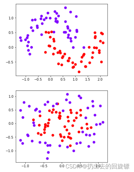
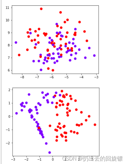
n_samples = 100
 
datasets = [
    make_moons(n_samples=n_samples, noise=0.2, random_state=0),
    make_circles(n_samples=n_samples, noise=0.2, factor=0.5, random_state=1),
    make_blobs(n_samples=n_samples, centers=2, random_state=5),#分簇的数据集
    make_classification(n_samples=n_samples,n_features = 2,n_informative=2,n_redundant=0, random_state=5)
                #n_features：特征数，n_informative：带信息的特征数，n_redundant：不带信息的特征数
    ]
 
Kernel = ["linear","poly","rbf","sigmoid"]
 
for X,Y in datasets:
    plt.figure(figsize=(5,4))
    plt.scatter(X[:,0],X[:,1],c=Y,s=50,cmap="rainbow")

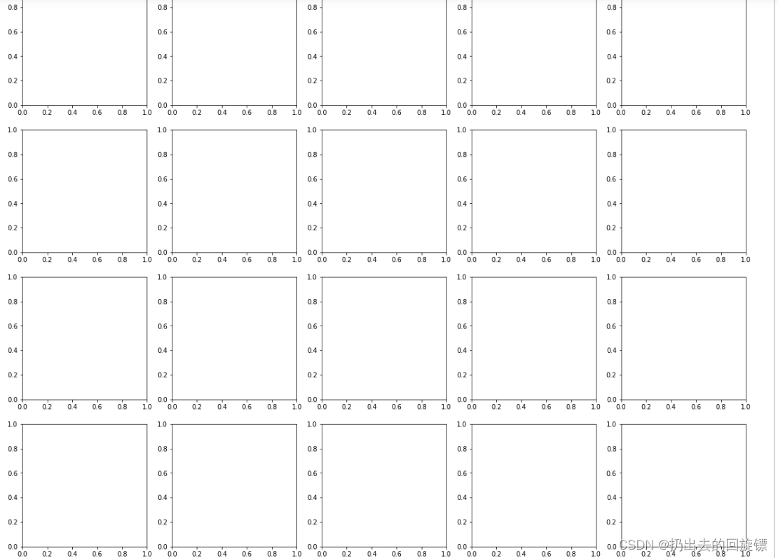
步骤二：构建子图，第一列为原始数据，后四列为模型学习结果

nrows = len(datasets)
ncols = len(Kernel)+1
fig, axes = plt.subplots(nrows, ncols,figsize=(20,16))

步骤三：函数绘图

nrows=len(datasets)
ncols=len(Kernel) + 1
fig, axes = plt.subplots(nrows, ncols,figsize=(20,16))

for ds_cnt, (X,Y) in enumerate(datasets):
    ax = axes[ds_cnt,0]
    if ds_cnt == 0:
        ax.set_title("Input data")
    ax.scatter(X[:,0],X[:,1],c=Y,zorder=10,cmap=plt.cm.Paired,edgecolors='k')
    ax.set_xticks(())
    ax.set_yticks(())
    
    for est_idx,kernel in enumerate(Kernel):
        ax = axes[ds_cnt,est_idx +1]
        clf = svm.SVC(kernel=kernel,gamma=2).fit(X,Y)
        score = clf.score(X,Y)
        ax.scatter(X[:,0],X[:,1],c=Y,zorder=10,cmap=plt.cm.Paired,edgecolors='k')
        #支持向量
        ax.scatter(clf.support_vectors_[:,0],clf.support_vectors_[:,1],s=50,facecolor='none',zorder=10,edgecolors='k')
        #决策边界
        x_min,x_max=X[:,0].min()-.5,X[:,0].max()+.5
        y_min,y_max=X[:,1].min()-.5,X[:,1].max()+.5
        XX, YY = np.mgrid[x_min:x_max:200j, y_min:y_max:200j]
        Z = clf.decision_function(np.c_[XX.ravel(), YY.ravel()]).reshape(XX.shape)
        ax.pcolormesh(XX,YY,Z>0,cmap=plt.cm.Paired)
        ax.contour(XX,YY,Z,colors=['k','k','k'],linestyles=['--','-','--'],levels=[-1,0,1])
        ax.set_xticks(())
        ax.set_yticks(())
        if ds_cnt ==0:
            ax.set_title(kernel)
        ax.text(0.95,0.06,('%.2f'%score).lstrip('0')
               ,size=15
               ,bbox=dict(boxstyle='round',alpha=0.8,facecolor='white')
               ,transform=ax.transAxes
               ,horizontalalignment='right')
        
plt.tight_layout()
plt.show()

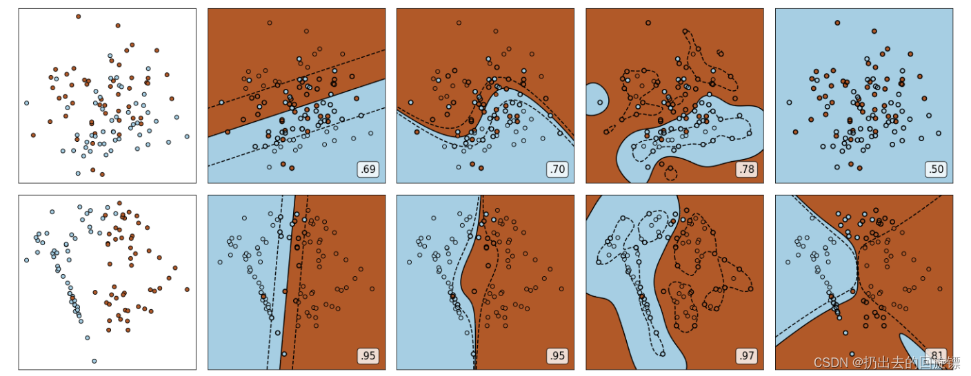
可以观察到，线性核函数和多项式核函数在非线性数据上表现会浮动，如果数据相对线性可分，则表现不错，如果是像环形数据那样彻底不可分的，则表现糟糕。在线性数据集上，线性核函数和多项式核函数即便有扰动项也可以表现不错，可见多项式核函数是虽然也可以处理非线性情况，但更偏向于线性的功能。Sigmoid核函数在非线性数据上强于两个线性核函数，但效果明显不如rbf，对扰动项的抵抗也比较弱，所以功能比较弱小，很少被用到。rbf基本在任何数据集上都表现不错，属于比较万能的核函数。

2.探索核函数的优势和缺陷

步骤一：导入库和数据

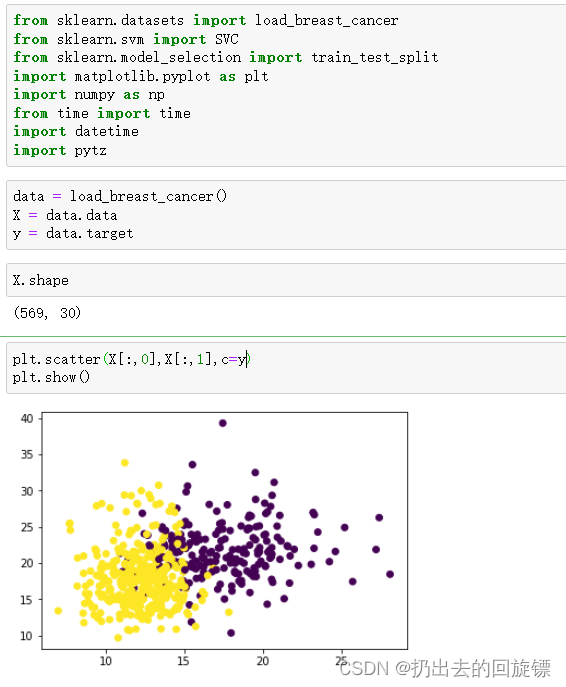
from sklearn.datasets import load_breast_cancer
from sklearn.svm import SVC
from sklearn.model_selection import train_test_split
import matplotlib.pyplot as plt
import numpy as np
from time import time
import datetime
import pytz

data = load_breast_cancer()
X = data.data
y = data.target

X.shape
plt.scatter(X[:,0],X[:,1],c=y)
plt.show()

步骤二：代入模型测试

Xtrain, Xtest, Ytrain, Ytest = train_test_split(X,y,test_size=0.3,random_state=420)
Kernel =  ["linear","poly",rbf","sigmoid"]

for kernel in Kernel:
    time0 = time()
    clf = SVC(kernel=kernel,
             gamma="auto"
             ,degree = 3
             ,cache_size=5000
             ).fit(Xtrain,Ytrain)
    print("The accuracy under kernel %s is %f"%(kernel,clf.score(Xtest,Ytest)))
    print(datetime.datetime.fromtimestamp(time()-time0,pytz.timezone('UTC')).strftime("%M:%S:%f"))

结果是运行poly模型时，一直无法完成。那么暂时去掉poly核函数

Xtrain, Xtest, Ytrain, Ytest = train_test_split(X,y,test_size=0.3,random_state=420)
Kernel =  ["linear","rbf","sigmoid"]

for kernel in Kernel:
    time0 = time()
    clf = SVC(kernel=kernel,
             gamma="auto"
             ,cache_size=5000
             ).fit(Xtrain,Ytrain)
    print("The accuracy under kernel %s is %f"%(kernel,clf.score(Xtest,Ytest)))
    print(datetime.datetime.fromtimestamp(time()-time0,pytz.timezone('UTC')).strftime("%M:%S:%f"))

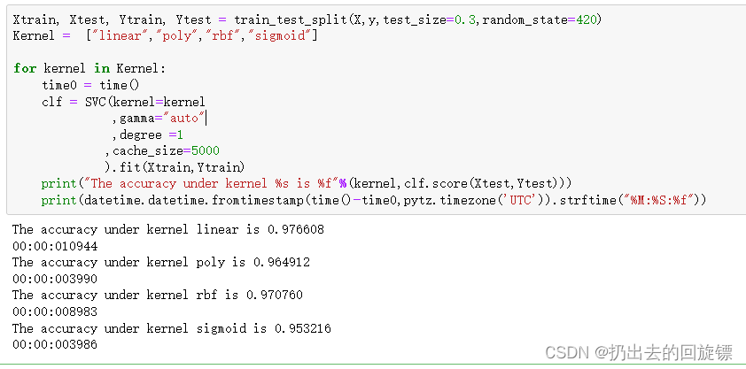
可以看到很轻松的跑出来了。虽然rbf和sigmoid概率预测很低，但用时远远小于linear。而且由于linear预测效果较好，那么将degree设置为1再次尝试poly核函数

Kernel =  ["linear","poly","rbf","sigmoid"]

for kernel in Kernel:
    time0 = time()
    clf = SVC(kernel=kernel
              ,gamma="auto"
              ,degree =1 
             ,cache_size=5000
             ).fit(Xtrain,Ytrain)
    print("The accuracy under kernel %s is %f"%(kernel,clf.score(Xtest,Ytest)))
    print(datetime.datetime.fromtimestamp(time()-time0,pytz.timezone('UTC')).strftime("%M:%S:%f"))

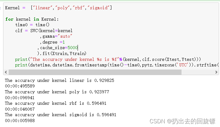
这次速度就很高了，而且poly精确性也和线性核函数接近。

步骤三：探索导致rbf和sigmoid结果偏低的可能

import pandas as pd
data = pd.DataFrame(X)
data.describe([0.01,0.05,0.1,0.25,0.5,0.75,0.9,0.99]).T

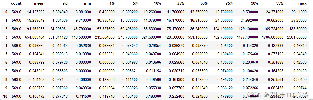
可以看到数据的量纲不一和偏态的问题很严重。所以可以归一化

from sklearn.preprocessing import StandardScaler
X = StandardScaler().fit_transform(X)
data = pd.DataFrame(X)
data.describe([0.01,0.05,0.1,0.25,0.5,0.75,0.9,0.99]).T

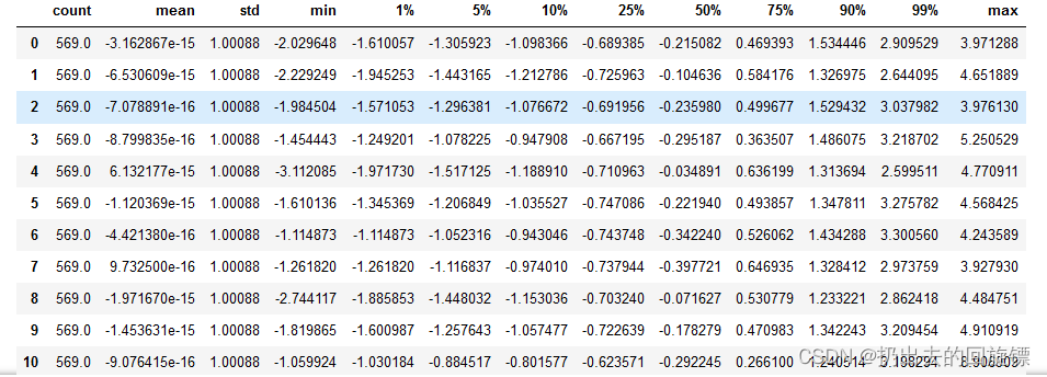
标准化后再次让SVM在核函数中遍历

Xtrain, Xtest, Ytrain, Ytest = train_test_split(X,y,test_size=0.3,random_state=420)
Kernel =  ["linear","poly","rbf","sigmoid"]

for kernel in Kernel:
    time0 = time()
    clf = SVC(kernel=kernel
              ,gamma="auto"
              ,degree =1 
             ,cache_size=5000
             ).fit(Xtrain,Ytrain)
    print("The accuracy under kernel %s is %f"%(kernel,clf.score(Xtest,Ytest)))
    print(datetime.datetime.fromtimestamp(time()-time0,pytz.timezone('UTC')).strftime("%M:%S:%f"))

可以看到，所有核函数特别是linear的运行时间都大大减少。同时rbf和sigmoid的效果也得到显著提高

结论：
1：线性核，尤其是多项式核函数在高次项时计算非常缓慢
2：rbf和多项式核函数都不擅长处理量纲不统一的数据集
3：SVM执行之前非常推荐先进行数据的无量纲化

步骤四：继续调整参数提高准确性

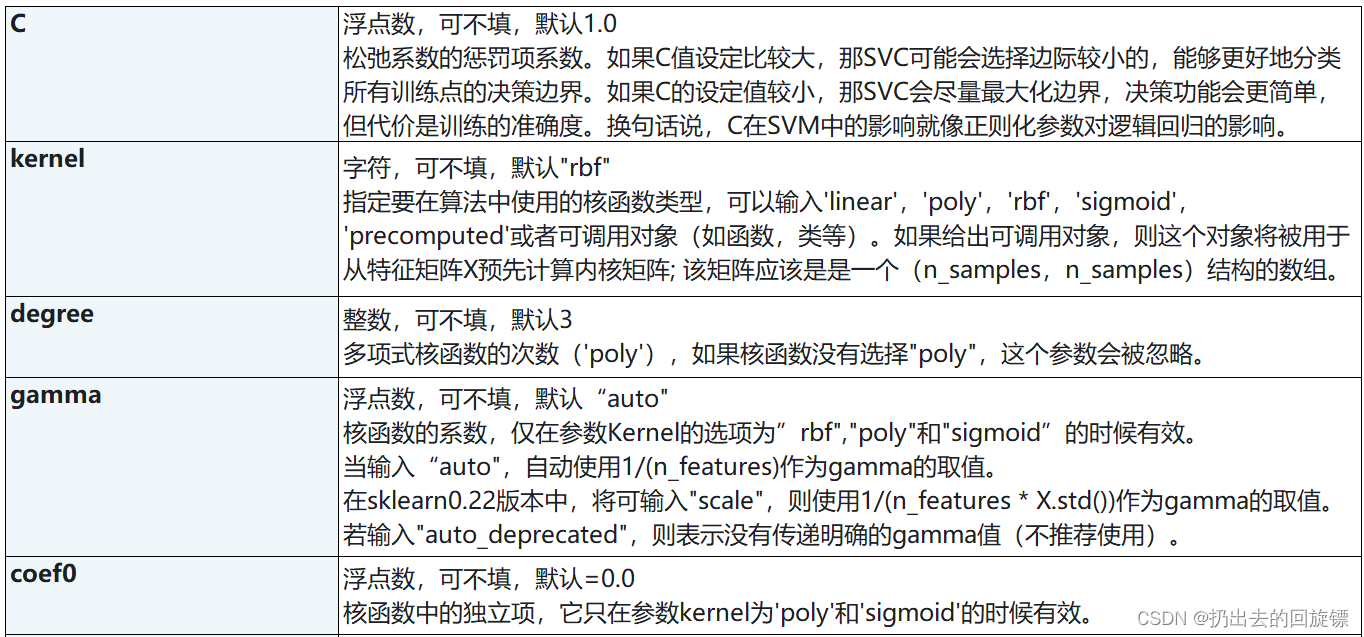
由之前核函数参数的表格可以知道，除了线性核函数以外，其他核函数还受参数gamma，degree以及coef0的影响。他们分别代表表达式中的$\gamma$,多项式中的次数$d$，常数项$r$

参数	含义
degree	整数，可不填，默认3 多项式核函数的次数（‘poly’），如果核函数没有选择"poly"，这个参数会被忽略
gamma	浮点数，可不填，默认“auto" 核函数的系数，仅在参数Kernel的选项为”rbf",“poly"和"sigmoid”的时候有效 输入“auto”，自动使用1/(n_features)作为gamma的取值 输入"scale"，则使用1/(n_features * X.std())作为gamma的取值 输入"auto_deprecated"，则表示没有传递明确的gamma值
coef0	浮点数，可不填，默认=0.0 核函数中的常数项，它只在参数kernel为’poly’和’sigmoid’的时候有效

由于数学问题太过复杂，这里采用学习曲线和网格搜索来寻找最佳参数

score = []
gamma_range = np.logspace(-10,1,50)
for i in gamma_range:
    clf = SVC(kernel="rbf",gamma=i,cache_size=5000).fit(Xtrain,Ytrain)
    score.append(clf.score(Xtest,Ytest))
print(max(score),gamma_range[score.index(max(score))])
plt.plot(gamma_range,score)
plt.show()

学习曲线与线性核函数之前准确率一样，应该是rbf核函数的极限了。由于多项式核函数有三个参数，所以使用网格搜索，同时注意不要分太多了防止计算量太大运行时间过长

from sklearn.model_selection import StratifiedShuffleSplit
from sklearn.model_selection import GridSearchCV
time0 = time()
gamma_range = np.logspace(-10,1,20)
coef0_range = np.linspace(0,5,10)
param_grid = dict(gamma = gamma_range
                 ,coef0=coef0_range)
cv =StratifiedShuffleSplit(n_splits=5,test_size=0.3,random_state=420)
grid = GridSearchCV(SVC(kernel = "poly",degree=1,cache_size=5000),
                   param_grid=param_grid,cv=cv)
grid.fit(X,y)
print("The best parameters are %s with a score of %0.5f" % (grid.best_params_, grid.best_score_))
print(datetime.datetime.fromtimestamp(time()-time0,pytz.timezone('UTC')).strftime("%M:%S:%f"))

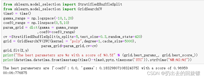
网格搜索为我们返回了参数coef0=0，gamma=0.18329807108324375，但整体的分数是0.96959，虽然比调参前略有提高，但依然没有超过线性核函数核rbf的结果。一般如果最初选择核函数的时候，多项式的结果不如rbf和线性核函数，就可以放弃它了，尝试调整rbf或者直接使用线性核函数。

步骤五：调整参数C

参数	含义
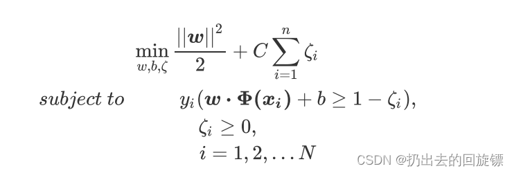
C	浮点数，默认1，必须大于等于0，可不填 松弛系数的惩罚项系数。如果C值设定比较大，那SVC可能会选择边际较小的，能够更好地分类所有训练点的决策边界，不过模型的训练时间也会更长。 如果C的设定值较小，那SVC会尽量最大化边界，决策功能会更简单，但代价是训练的准确度。换句话说，C在SVM中的影响就像正则化参数对逻辑回归的影响

为什么要引入C？

当两组数据完全线性可分，找出一个决策边界使得训练集上的分类误差为0，这两种数据就被称为是存在”硬间隔“的
当两组数据几乎是完全线性可分的，但决策边界在训练集上存在较小的训练误差，这两种数据就被称为是存在”软间隔“

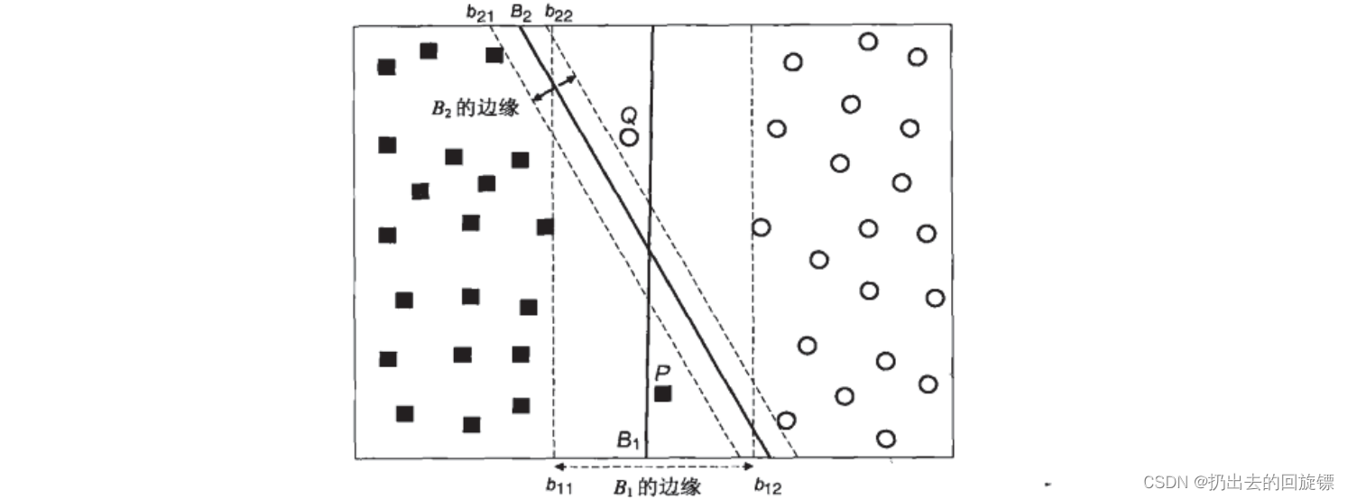
如图表示，虽然边际大的B1没有正确划分所有的数据。但不能认为此事B2就一定是一条更好的边界。需要找出一个“最大边际”与“被分错的样本数量”之间的平衡

引入C的方式

原始判别函数为：
$$w\cdot x_i+b\ge 1,if{y}_i=1$$
$$w\cdot x_i+b\le -1,if{y}_i=-1$$
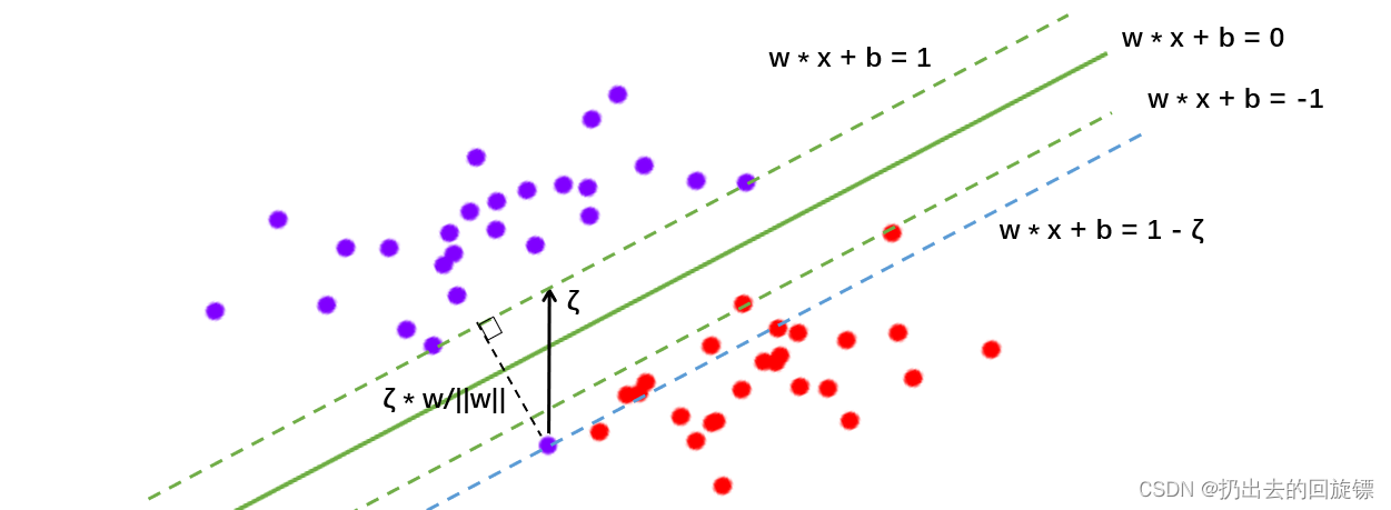
引入松弛系数$\zeta$后的判别函数：
$$w\cdot x_i+b\ge 1-{\zeta }_i,if{y}_i=1$$
$$w\cdot x_i+b\le -1+{\zeta }_i,if{y}_i=-1$$
实际上就是将虚线超平面往图像的上方和下方平移，平移后同时会分错一系列别的点。所以必须再添加一个惩罚项，用来惩罚具有巨大松弛系数C的决策超平面。此时的损失函数表示为：

拉格朗日函数为：（u为第二个拉格朗日乘数）

拉格朗日对偶函数为：

公式中现在唯一的新变量，松弛系数的惩罚力度C，由参数C来进行控制

通过学习曲线调整C的值

score = []
C_range = np.linspace(0.01,30,50)
for i in C_range:
    clf = SVC(kernel="linear",C=i,cache_size=5000).fit(Xtrain,Ytrain)
    score.append(clf.score(Xtest,Ytest))
print(max(score),C_range[score.index(max(score))])
plt.plot(C_range,score)
plt.show()

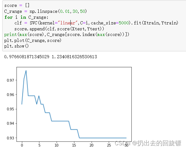
linear的最大值和之前求得一样，根据图像也可以得出之前的就是最佳值

score = []
C_range = np.linspace(0.01,30,50)
for i in C_range:
    clf = SVC(kernel="rbf",C=i
              ,gamma=0.012067926406393264
              ,cache_size=5000).fit(Xtrain,Ytrain)
    score.append(clf.score(Xtest,Ytest))
print(max(score),C_range[score.index(max(score))])
plt.plot(C_range,score)
plt.show()

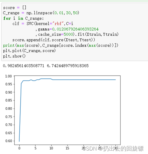
继续细分

score = []
C_range = np.linspace(5,7,50)
for i in C_range:
    clf = SVC(kernel="rbf",C=i
              ,gamma=0.012067926406393264
              ,cache_size=5000).fit(Xtrain,Ytrain)
    score.append(clf.score(Xtest,Ytest))
print(max(score),C_range[score.index(max(score))])
plt.plot(C_range,score)
plt.show()

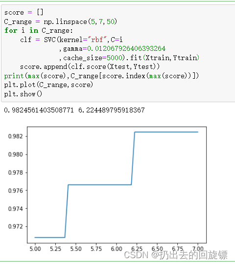
此时找到最优解，准确率最高的是rbf

附录

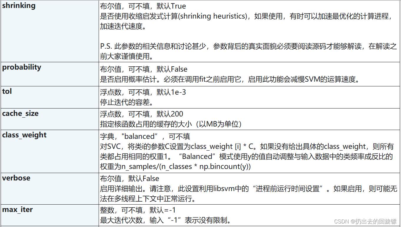
svc参数列表



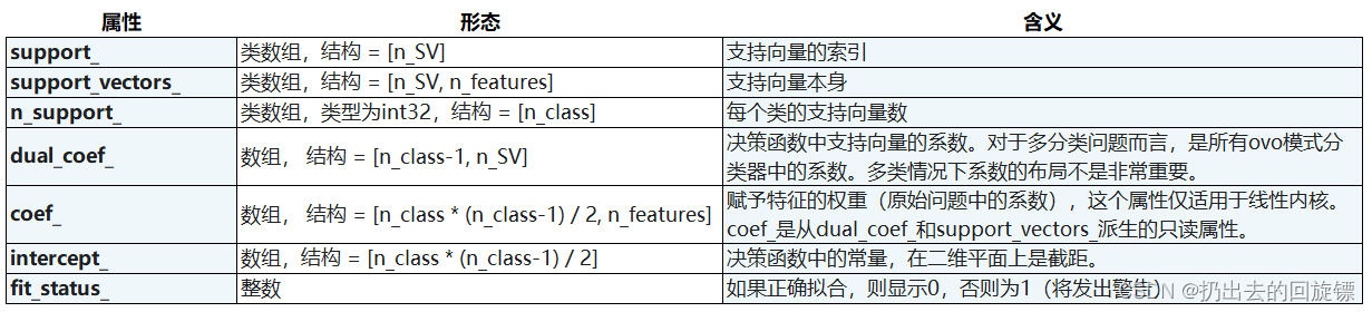
SVC属性列表

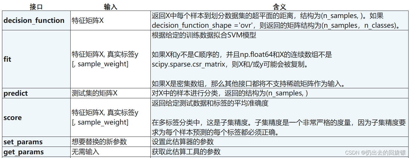
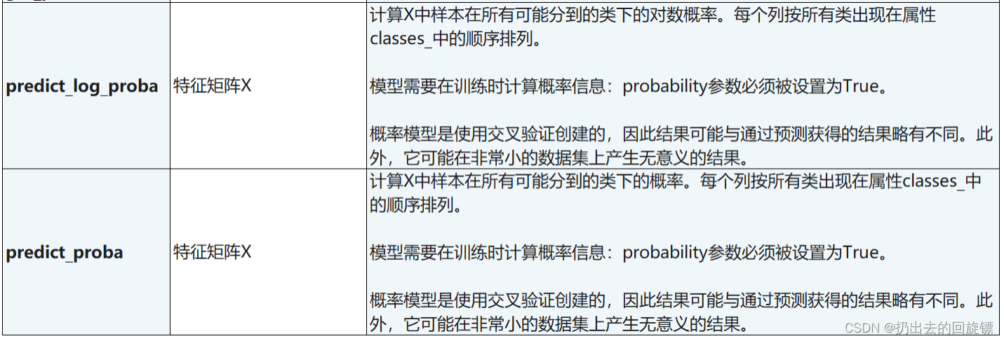
SVC接口列表