


这个月的目标是先学习船舶轨迹压缩的相关算法,这周看的主要是DP算法
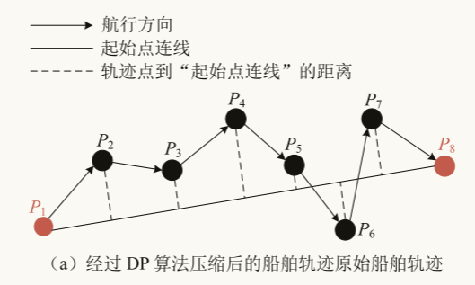
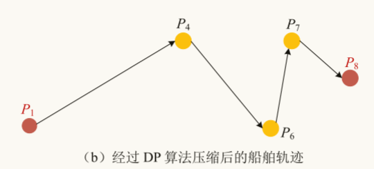
DP算法由 David Douglas和 Thomas Peucker 于 1973年首次提出,是一种经典的线性元素简化算法。在处理大量冗余几何数据点时,主要使用 DP算法。该算法在压缩轨迹的同时,还能保留轨迹的形状特征 。算法整体的思路,简单来说,就是通过设置压缩阈值来对轨迹进行简化。具体的思路为:假设航行轨迹由8个点到
组成,将起点与终点连线,再计算中间航迹点到这条直线的距离,依次比较这些距离,得到最大距离
,随后将
与预设阈值
进行比较,若
.则中间点要全部舍去;若
,则把这条轨迹分成两部分。然后再对这两部分轨迹分别执行上述操作,依次迭代,直到压缩完成,就可以得到最终轨迹。如图(a)(b)所示
下边是DP算法的代码:
import numpy as np
from math import sqrt
import matplotlib.pyplot as plt
class DouglasPeucker(object):
"""该类实现了道格拉斯 - 普克(Douglas Peucker)算法,用于对轨迹进行空间压缩。
用户需要指定压缩阈值。
"""
def __init__(self):
pass
def compress(self, Q, delta):
"""关键字参数:
Q -- 轨迹点集 (矩阵形式,每行是一个点的坐标)
delta -- 压缩阈值
"""
indicies = self._douglas_peucker(Q, 0, len(Q) - 1, delta)
compressed_Q = Q[indicies]
return compressed_Q
def _douglas_peucker(self, Q, s, t, delta):
"""返回道格拉斯 - 普克简化轨迹的下标
关键字参数:
Q -- 查询轨迹(矩阵)
s -- 起始位置
t -- 结束位置
delta -- 压缩阈值
"""
indecies = []
dmax = -float('inf')
for i in range(s + 1, t):
d = self._perpendicular_dist(Q, s, t, i)
if d > dmax:
dmax = d
idx = i
if dmax > delta:
L1 = self._douglas_peucker(Q, s, idx, delta)
L2 = self._douglas_peucker(Q, idx, t, delta)
[indecies.append(x) for x in L1]
indecies.pop(-1) # 移除重复元素
[indecies.append(x) for x in L2]
else:
indecies.append(s)
indecies.append(t)
return indecies
def _perpendicular_dist(self, Q, s, t, i):
x0, y0, x1, y1, x, y = Q[s][0], Q[s][1], Q[t][0], Q[t][1], Q[i][0], Q[i][1]
# 公式来源: http://mathworld.wolfram.com/Point-LineDistance2-Dimensional.html
return abs((x1 - x0) * (y0 - y) - (x0 - x) * (y1 - y0)) / sqrt((x1 - x0) * (x1 - x0) + (y1 - y0) * (y1 - y0))
if __name__ == "__main__":
dp = DouglasPeucker()
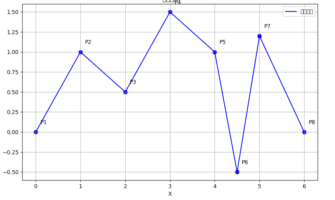
# 预设轨迹点
Q = np.array([
[0, 0],
[1, 1],
[2, 0.5],
[3, 1.5],
[4, 1],
[4.5, -0.5],
[5, 1.2],
[6, 0]
])
delta = 0.5 # 压缩阈值,可调整
# 可视化原始轨迹
plt.figure(figsize=(10, 6))
plt.plot(Q[:, 0], Q[:, 1], 'b-', label='原始轨迹')
plt.scatter(Q[:, 0], Q[:, 1], color='b', s=50)
for i, point in enumerate(Q):
plt.annotate(f'P{i + 1}', xy=point, xytext=(point[0] + 0.1, point[1] + 0.1))
plt.title('原始轨迹')
plt.xlabel('X')
plt.ylabel('Y')
plt.legend()
plt.grid(True)
plt.savefig('original_trajectory.png')
plt.show()
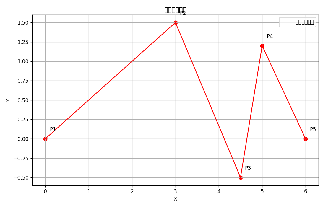
# 进行轨迹压缩
compressed_Q = dp.compress(Q, delta)
# 可视化压缩后的轨迹
plt.figure(figsize=(10, 6))
plt.plot(compressed_Q[:, 0], compressed_Q[:, 1], 'r-', label='压缩后的轨迹')
plt.scatter(compressed_Q[:, 0], compressed_Q[:, 1], color='r', s=50)
for i, point in enumerate(compressed_Q):
plt.annotate(f'P{i + 1}', xy=point, xytext=(point[0] + 0.1, point[1] + 0.1))
plt.title('压缩后的轨迹')
plt.xlabel('X')
plt.ylabel('Y')
plt.legend()
plt.grid(True)
plt.savefig('compressed_trajectory.png')
plt.show()实验结果:
这里为了方便实验结果的呈现,预设了轨迹点。下方为导入文件中数据的代码:
import numpy as np
from math import sqrt
import matplotlib.pyplot as plt
class DouglasPeucker(object):
"""该类实现了道格拉斯 - 普克(Douglas Peucker)算法,用于对轨迹进行空间压缩。
用户需要指定压缩阈值。
"""
def __init__(self):
pass
def compress(self, unfn, wfn, delta):
"""关键字参数:
unfn -- 待压缩的轨迹数据文件
wfn -- 压缩后的轨迹数据文件
delta -- 压缩阈值
"""
Q = np.genfromtxt(unfn, delimiter=',')
indicies = self._douglas_peucker(Q, 0, len(Q) - 1, delta)
with open('log.txt', 'w') as f:
f.write('文件压缩总结: ' + unfn + '\n')
f.write('\t- 压缩前有 ' + str(len(Q)) + ' 个数据点\n')
f.write('\t- 压缩后有 ' + str(len(indicies)) + ' 个数据点\n')
f.write('\t- 压缩率: ' + str(1 - float(len(indicies)) / len(Q)) + '\n')
with open(wfn, 'w') as f:
for i in indicies:
f.write(str(Q[i][0]) + ',' + str(Q[i][1]) + '\n')
return Q, indicies
def _douglas_peucker(self, Q, s, t, delta):
"""返回道格拉斯 - 普克简化轨迹的下标
关键字参数:
Q -- 查询轨迹(矩阵)
s -- 起始位置
t -- 结束位置
delta -- 压缩阈值
"""
indecies = []
dmax = -float('inf')
for i in range(s + 1, t):
d = self._perpendicular_dist(Q, s, t, i)
if d > dmax:
dmax = d
idx = i
if dmax > delta:
L1 = self._douglas_peucker(Q, s, idx, delta)
L2 = self._douglas_peucker(Q, idx, t, delta)
[indecies.append(x) for x in L1]
indecies.pop(-1) # 移除重复元素
[indecies.append(x) for x in L2]
else:
indecies.append(s)
indecies.append(t)
return indecies
def _perpendicular_dist(self, Q, s, t, i):
x0, y0, x1, y1, x, y = Q[s][0], Q[s][1], Q[t][0], Q[t][1], Q[i][0], Q[i][1]
# 公式来源: http://mathworld.wolfram.com/Point-LineDistance2-Dimensional.html
return abs((x1 - x0) * (y0 - y) - (x0 - x) * (y1 - y0)) / sqrt((x1 - x0) * (x1 - x0) + (y1 - y0) * (y1 - y0))
if __name__ == "__main__":
dp = DouglasPeucker()
# 设置压缩阈值
delta = 0.006
Q = np.genfromtxt('Data/Uncompressed/cycling_trajectory_20120916.txt', delimiter=',')
indicies = dp._douglas_peucker(Q, 0, len(Q) - 1, delta)
print(len(Q), '个数据点在压缩前')
print(len(indicies), '个数据点在压缩后')
print('压缩率:', 1 - float(len(indicies)) / len(Q))
Q, indicies = dp.compress('Data/Uncompressed/cycling_trajectory_20120916.txt',
'Data/Compressed/compressed_cycling_trajectory_20120916.txt', delta)
# 可视化原始轨迹
plt.figure(figsize=(10, 6))
plt.plot(Q[:, 0], Q[:, 1], 'b-', label='原始轨迹')
plt.title('原始轨迹')
plt.xlabel('X')
plt.ylabel('Y')
plt.legend()
plt.grid(True)
plt.savefig('original_trajectory.png')
plt.show()
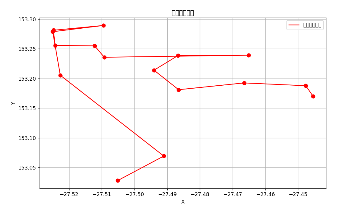
# 可视化压缩后的轨迹
plt.figure(figsize=(10, 6))
compressed_Q = Q[indicies]
plt.plot(compressed_Q[:, 0], compressed_Q[:, 1], 'r-', label='压缩后的轨迹')
plt.scatter(compressed_Q[:, 0], compressed_Q[:, 1], color='r', s=50)
plt.title('压缩后的轨迹')
plt.xlabel('X')
plt.ylabel('Y')
plt.legend()
plt.grid(True)
plt.savefig('compressed_trajectory.png')
plt.show()
实验结果:
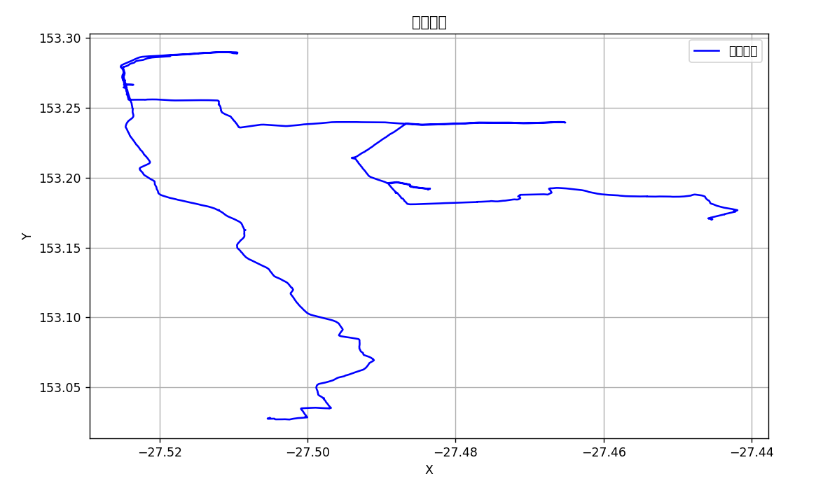
 2684 个数据点在压缩前
16 个数据点在压缩后
参考文献:
[1] 张仕泽.基于 AIS数据的船舶典型轨迹提取方法研究[D]. 大连:大连海事大学,2024.
欢迎留言,欢迎指正:)


 被折叠的 条评论
为什么被折叠?
被折叠的 条评论
为什么被折叠?
 到【灌水乐园】发言


