《模式分类》第二版 第二章课后编程题

这篇博客所有的数据和代码都在GitHub上可以找到，特别是编程题需要的.mat文件需要到Github上下载。下面我会把题目要求、代码和实验结果贴出来，如果有什么错误的地方，希望大家可以提出来。

1.下面的几道题可能会用到如下的程序：
（a）写一个程序产生服从d维正态分布$N(\mu, \Sigma)$的随机样本。
（b）写一个程序计算一给定正态分布及先验概率$P(\omega_i)$的判别函数($g_i(x) = -\frac{1}{2}(x - \mu_i)^t\Sigma_i^{-1}(x - \mu_i) - \frac{d}{2}ln2\pi - \frac{1}{2}ln|\Sigma_i| + lnP(\omega_i)$)。
（c）写一个程序计算任意两点间的欧氏距离。
（d）在给定协方差矩阵$\Sigma$的情况条件下，写一个程序计算任意一点x到均值$\mu$间的Mahalanobis距离。

CH2_1_a.m: Generate random vectors from the multivariate normal distribution.

function r = CH2_1_a(u, sigma, n)
% function r = CH2_1_a(u, sigma, n)
% Generate random vectors from the multivariate normal distribution.
% Inputs:
%   u     - Mean of distribution
%   sigma - Covariance matrix of distribution
%   n     - Number of vectors
%
% Outputs:
%   r     - Matrix of random vectors

r = mvnrnd(u, sigma, n);
end

CH2_1_a_test.m: Generate two normal distributions and plot.

% generate a normal distribution
u1 = [0, 0];
sigma1 = [2 0; 0 2];
r1 = CH2_1_a(u1, sigma1, 500);
plot(r1(:, 1), r1(:, 2), 'r+');
hold on;

% generate another normal distribution
u2 = [5, 5];
sigma2 = [.5 0; 0 2];
r2 = CH2_1_a(u2, sigma2, 500);
plot(r2(:, 1), r2(:, 2), '*');
xlabel('x1'), ylabel('x2');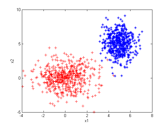

CH2_1_b.m: Discriminant function of a normal distribution given prior probability.

function g = CH2_1_b(x, u, sigma, P)
% function g = CH2_1_b(x, u, sigma, P)
% Discriminant function of a normal distribution given prior probability.
% Inputs:
%   x     - Input vector
%   u     - Mean of distribution
%   sigma - Covariance matrix of distribution
%   P     - Prior probability
%
% Ouputs:
%   g     - Discriminant result 

g = -0.5*(x - u)'*inv(sigma)*(x - u) - size(u, 1)/2.0*log(2*pi) - 0.5*log(det(sigma)) + log(P);
end

CH2_1_c.m: Calculate the Euclidean distance between two vectors.

function E_dist = CH2_1_c(x1, x2)
% function E_dist = CH2_1_c(x1, x2)
% Calculate the Euclidean distance between two vectors.
% Inputs:
%   x1     - Vector x1
%   x2     - Vector x2
%
% Outputs:
%   E_dist - Euclidean distance

E_dist = sqrt(sum((x1 - x2).^2));
end

CH2_1_d.m: Calculate the Mahalanobis distance of a vector.

function M_dis = CH2_1_d(x, u, sigma)
% function M_dis = CH2_1_d(x, u, sigma)
% Calculate the Mahalanobis distance of a vector.
% Inputs:
%   x      - Input Vector
%   u      - Mean of distribution
%   sigma  - Covariance matrix of distribution
%
% Outputs:
%   M_dis  - Mahalanobis distance

M_dis = sqrt((x - u)'*inv(sigma)*(x - u));
end

2.参考上机练习1（b），并考虑将上面表格中的10个样本点进行分类的问题，假设分布是正态的。
（a）假设前面两个类别的先验概率相等($P(\omega_1) = P(\omega_2) = 1/2$，且$P(\omega_3) = 0)$，仅利用$x_1$特征值为这两类判别设计一个分类器。
（b）确定样本的经验训练误差，即误分点的百分比。
（c）利用Bhattacharyya界来界定对该分布所产生的新模式进行分类会产生的误差。
（d）现在利用两个特征值$x_1$和$x_2$，重复以上各步。
（e）利用所有3个特征值重复以上各步。
（f）讨论所得的结论。特别是，对于一有限的数据集，是否有可能在更高的数据维数下经验误差会增加？ 可能

CH2_2.m: Generate classification model of two classes, then calculate the classification error and the Bhattacharyya bound.

function [model, error, Bbound] = CH2_2(patterns, targets, c1, c2, P1, P2, dim)
% function [model, error, Bbound] = CH2_2(patterns, targets, c1, c2, P1, P2, dim)
% Generate classification model of two classes, then calculate the classification
% error and the Bhattacharyya bound.
% Inputs:
%   patterns - Input matrix
%   targets  - Input matrix classes
%   c1       - Class1
%   c2       - Class2
%   P1       - Prior probability of c1
%   P2       - Prior probability of c2
%   dim      - Dimensions of input vector
%
% Outputs:
%   model    - Classification model
%   error    - Classification error
%   Bbound   - Bhattacharyya bound

%% Generate classification model
% matrices of two classes
x1 = patterns(1:dim, targets == c1);
x2 = patterns(1:dim, targets == c2);
% mean of two matrices
u1 = mean(x1, 2);
u2 = mean(x2, 2);
% covariance matrix of two matrices
sigma1 = cov(x1');
sigma2 = cov(x2');
% generate model
model.u1 = u1;
model.u2 = u2;
model.sigma1 = sigma1;
model.sigma2 = sigma2;
model.P1 = P1;
model.P2 = P2;

%% Calculate the classification error
col1 = size(x1, 2);
col2 = size(x2, 2);
result1 = zeros(col1, 1);
result2 = zeros(col2, 1);
% classification result
for i = 1:col1
    if CH2_1_b(x1(:, i), model.u1, model.sigma1, model.P1) >=  CH2_1_b(x1(:, i), model.u2, model.sigma2, model.P2)
        result1(i) = c1;
    else
        result1(i) = c2;
    end
end
for i = 1:col2
    if CH2_1_b(x2(:, i), model.u2, model.sigma2, model.P2) >=  CH2_1_b(x2(:, i), model.u1, model.sigma1, model.P1)
        result2(i) = c2;
    else
        result2(i) = c1;
    end
end
% classification error
error_num = size(find(result1 == c2), 1) + size(find(result2 == c1), 1);
error = error_num/(col1 + col2);

%% Bhattacharyya bound
Bbound = Bhattacharyya(u1, sigma1, u2, sigma2, P1);

CH2_2_test.m: Plot classification error and Bhattacharyya bound.

load CH2.mat
error_vec = zeros(3, 1);
Bbound_vec = zeros(3, 1);
% calculate classification error and Bhattacharyya bound
for i = 1:3
    [model, error, Bbound] = CH2_2(patterns, targets, 1, 2, 0.5, 0.5, i);
    model_cell{i} = model;
    error_vec(i) = error;
    Bbound_vec(i) = Bbound;
end
% plot 
plot(1:3, error_vec, '--ro', 1:3, Bbound_vec, '-g*');
xlabel('dim');
ylabel('error');
legend('classification error', 'Bhattacharyya bound');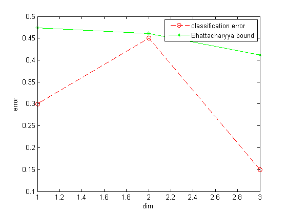

3.对于类别$\omega_1$和$\omega_3$重复上机题2。

CH2_3.m: Plot classification error and Bhattacharyya bound.

load CH2.mat
error_vec = zeros(3, 1);
Bbound_vec = zeros(3, 1);
% calculate classification error and Bhattacharyya bound
% same to CH2_2_test
% modify two classes and two prior probabilities
for i = 1:3
    [model, error, Bbound] = CH2_2(patterns, targets, 1, 3, 0.5, 0.5, i);
    model_cell{i} = model;
    error_vec(i) = error;
    Bbound_vec(i) = Bbound;
end
% plot 
plot(1:3, error_vec, '--ro', 1:3, Bbound_vec, '-g*');
xlabel('dim');
ylabel('error');
legend('classification error', 'Bhattacharyya bound');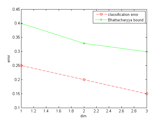

4.考虑上机题2中的3个类别，设$P(\omega_i) = 1/3$。
（a）以下各测试点与上机练习2中各类别均值间的Mahalanobis距离分别是多少：$(1, 2, 1)^t, (5, 3, 2)^t, (0, 0, 0)^t, (1, 0, 0)^t$。
（b）对以上各点进行分类。
（c）若设$P(\omega_1) = 0.8, P(\omega_2) = P(\omega_3) = 0.1$，再对以上测试点进行分类。

CH2_4.m: Calculate the Mahalanobis distance with three classes, then classify the vectors.

function [M_dist, class] = CH2_4(x, patterns, targets, P)
% function [M_dist, class] = CH2_4(x, patterns, targets, P1, P2, P3)
% Calculate the Mahalanobis distance with three classes, then classify the
% vectors.
% Inputs:
%   x         - Input vector
%   patterns  - Input matrix
%   targets   - Input matrix classes
%   P         - Prior probability of class 1,2,3
% 
% Outputs:
%   M_dist    - Mahalanobis distance
%   class     - classification result

%% Mahalanobis distance
m = size(patterns, 1);
for i = 1:m
   p = patterns(:, targets == i);
   u{i} = mean(p, 2);
   sigma{i} = cov(p');
end
for i = 1:m
    M_dist(i) = CH2_1_d(x, u{i}, sigma{i});
end

%% classification
class = 0; max_g = -Inf;
for i = 1:m
    g = CH2_1_b(x, u{i}, sigma{i}, P(i));
    if g > max_g
        class = i;
        max_g = g;
    end
end

end

CH2_4_test.m: Test CH2_4.m with four vectors.

load CH2.mat
v = [1 2 1; 5 3 2; 0 0 0; 1 0 0]';
%% P = [1/3 1/3 1/3]
P = [1/3 1/3 1/3];
fprintf('The prior probability of three classes is : [1/3 1/3 1/3]\n');
for i = 1:size(v, 2)
    x = v(:, i);
    [M_dist, class] = CH2_4(x, patterns, targets, P);
    fprintf('The Mahalanobis distance between vector %d and three classes is %f, %f, %f\n', ...
        i, M_dist(1), M_dist(2), M_dist(3));
    fprintf('Vector %d belongs to class %d\n\n', i, class);
end
fprintf('\n\n\n');
%% P = [0.8 0.1 0.1]
P = [0.8 0.1 0.1];
fprintf('The prior probability of three classes is : [0.8 0.1 0.1]\n');
for i = 1:size(v, 2)
    x = v(:, i);
    [M_dist, class] = CH2_4(x, patterns, targets, P);
    fprintf('The Mahalanobis distance between vector %d and three classes is %f, %f, %f\n', ...
        i, M_dist(1), M_dist(2), M_dist(3));
    fprintf('Vector %d belongs to class %d\n\n', i, class);
end

5.通过以下步骤说明这样一个事实：大量独立的随机变量的平均将近似为一高斯分布。
（a）写一个程序，从一均匀分布U($x_l, x_u$)中产生n个随机整数。（有些计算机系统在其函数库中包含了这样的函数调用。）
（b）现在写一个程序，从范围$-100\leq x_l < x_u \leq +100$中随机取$x_l$和$x_u$，以及在范围$0 < n \leq 1000$中随机取n的值（样本数）。
（c）通过以上所述的方式累计产生$10^4$个样本点，并绘制一直方图。
（d）计算该直方图的均值和标准差，并绘图。
（e）对于$10^5$和$10^6$个样本点分别重复以上步骤，讨论所得结论。

CH2_5.m: The script is to prove that the average of a large number of independent random variables follows Gauss distribution.

% The script is to prove that the average of a large number of
% independent random variables follows Gauss distribution.

% 10^4, 10^5, 10^6 samples
% 1. randomly pick xl and xu, -100 <= xl < xu <= 100
% 2. randomly pick n, 0 <= n <= 1000
% 3. randomly pick n numbers from [xl xu]
% 4. calculate the average of the n numbers
for i = 4:6
    h = zeros(1, 0);
    y = zeros(1, 0);
    while size(h, 2) < 10^i
       x = randi([-100 100], 1, 2);
       if min(x) == max(x)
           continue;
       end
       xl = min(x);
       xu = max(x);
       n = randi([0 1000], 1, 1);
       v = randi([xl xu], 1, n);
       y = [y mean(v)];
       h = [h y];
    end
    % hist
    subplot(2, 2, i - 3);
    hist(y, 50);
    xlabel('x'), ylabel('num of x');
    title(['10^',num2str(i),' samples']);
    fprintf('10^%d samples:\n', i);
    fprintf('mean:%f  std:%f\n\n', mean(y), std(y));
end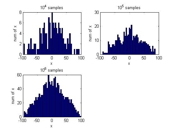

6.根据以下步骤测试经验误差是如何接近或不接近Bhattacharyya界的：
（a）写一个程序产生d维空间的样本点，服从均值为$\mu$和协方差矩阵$\Sigma$的正态分布。
（b）考虑正态分布
$p(x|\omega_1) \sim N(\begin{pmatrix} 1 \\ 0 \end{pmatrix}, I)$和$p(x|\omega_2) \sim N(\begin{pmatrix} -1 \\ 0 \end{pmatrix}, I)$
且$P(\omega_1) = P(\omega_2) = 0.5$。说明贝叶斯判决边界。
（c）产生n = 100个点（50个$\omega_1$类点点，50个$\omega_2$类的点），并计算经验误差。
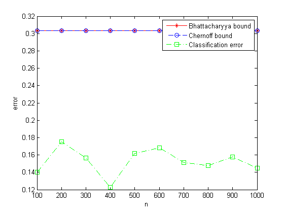
（d）对于不断增加的n值重复以上步骤，$100 \leq n \leq 1000$，步长量为100，并绘出所得的经验误差。
（e）讨论所得的结论。特别是，经验误差是否可能比Bhattacharyya或Chernoff界还大。 可能

CH2_6.m: Calculate the classification error of two classes.

function [error, Bbound, Cbound] = CH2_6(u1, sigma1, u2, sigma2, P1, P2)
% function error = CH2_6(u1, sigma1, u2, sigma2, P1, P2)
% Calculate the classification error of two classes.
% Inputs:
%   u1     - Mean of class1
%   sigma1 - Covariance matrix of class1
%   u2     - Mean of class2
%   sigma2 - Covariance matrix of class2
%   P1     - Prior probability of class1
%   P2     - Prior probability of class2
%
% Outputs:
%   error  - Classification error
%   Bbound - Bhattacharyya bound
%   Cbound - Chernoff bound

%% plot Gauss distribution
% Gauss distribution
[x1_1, x1_2] = meshgrid(linspace(-4, 6, 100)', linspace(-5, 5, 100)');
x1 = [x1_1(:) x1_2(:)];
p1 = P1*mvnpdf(x1, u1', sigma1);
surf(x1_1, x1_2, reshape(p1, 100, 100));
hold on;
[x2_1, x2_2] = meshgrid(linspace(-6,4,100)', linspace(-5,5,100)');
x2 = [x2_1(:) x2_2(:)];
p2 = P2*mvnpdf(x2, u2', sigma2);
surf(x2_1, x2_2, reshape(p2, 100, 100));
xlabel('x1'), ylabel('x2'), zlabel('p');
% Obviously, surf x1 = 0 is the Bayes decision boundary.

%% classification error, Bhattacharyya bound, Chernoff bound
figure;
Bbound = Bhattacharyya(u1, sigma1, u2, sigma2, P1);
Cbound = Chernoff(u1, sigma1, u2, sigma2, P1);
for n = 100:100:1000
    r1 = CH2_1_a(u1, sigma1, n/2);
    r2 = CH2_1_a(u2, sigma2, n/2);
    % error1_2: number of class1 misclassified to class2
    % error2_1: number of class2 misclassified to class1
    error1_2 = 0;
    error2_1 = 0;
    for i = 1:size(r1, 1)
        % class1 misclassified to class2
        if(CH2_1_b(r1(i, :)', u1, sigma1, P1) < CH2_1_b(r1(i, :)', u2, sigma2, P2))
            error1_2 = error1_2 + 1;
        end
        % class2 misclassified to class1
        if(CH2_1_b(r2(i, :)', u2, sigma2, P2) < CH2_1_b(r2(i, :)', u1, sigma1, P1))
            error2_1 = error2_1 + 1;
        end
    end
    error(n/100) = (error1_2 + error2_1)/n;
end
plot(100:100:1000, Bbound*ones(1, 10), '-r*', ...
    100:100:1000, Cbound*ones(1, 10), '--bo', ...
    100:100:1000, error, '-.gs');
xlabel('n'), ylabel('error');
legend('Bhattacharyya bound', 'Chernoff bound', 'Classification error');
end

CH2_6_test.m: Test CH2_6.m.

u1 = [1 0]';
sigma1 = [1 0; 0 1];
u2 = [-1 0]';
sigma2 = [1 0; 0 1];
[error, Bbound, Cbound] = CH2_6(u1, sigma1, u2, sigma2, 0.5, 0.5);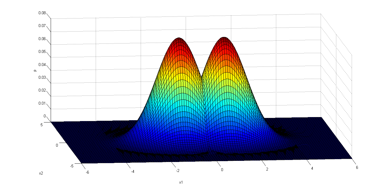

7.考虑两个一维正态分布$p(x|\omega_1) \sim N(-0.5, 1)$及$p(x|\omega_2) \sim N(+0.5, 1)$，且$P(\omega_1) = P(\omega_2) = 0.5$。
（a）计算一个贝叶斯分类器的Bhattacharyya误差界。
（b）用一个误差函数$erf (\cdot)$的形式表示实际误差率。$(1 - erf(\sqrt {2}/4))/2$
（c）通过数值积分（或其他方式）估计此实际误差，精确到4位有效数字。
（d）分别产生每类10个样本点，并确定用以上贝叶斯分类器进行分类时的经验误差。（必须对每一套数据重新计算判决边界）
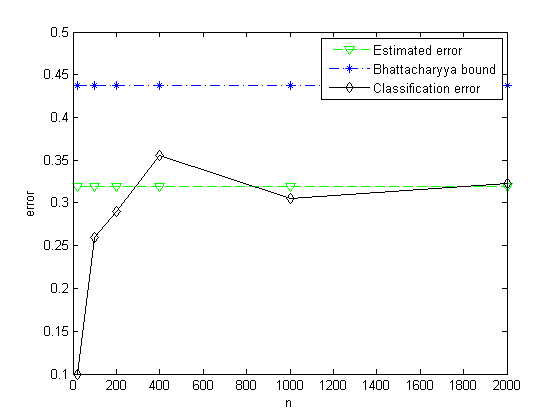
（e）通过重复前面的步骤，并分别从两种分布中各取50、100、200、500及1000个样本点，绘制出经验误差作为取自两种分布的样本点数的函数图。比较渐近于实际误差的经验误差同Bhattacharyya误差界。

CH2_7.m: Calculate the Bhattacharyya bound, estimated error and a series of classification error of two Gauss distribution.

function [Eerror, Bbound, Cerror] = CH2_7(u1, sigma1, u2, sigma2, P1, P2)
% function [Eerror, Bbound, Cerror] = CH2_7(u1, sigma1, u2, sigma2, P1, P2)
% Calculate the Bhattacharyya bound, estimated error and a
% series of classification error of two Gauss distribution.
% Inputs:
%   u1     - Mean of class1
%   sigma1 - Covariance matrix of class1
%   u2     - Mean of class2
%   sigma2 - Covariance matrix of class2
%   P1     - Prior probability of class1
%   P2     - Prior probability of class2
%
% Outputs:
%   Eerror - Estimated error
%   Bbound - Bhattacharyya bound
%   Cerror - Classification error

%% calculate the curve intersection point
eq1 = ['y = ' num2str(P1) '*1/sqrt(2*pi*' num2str(sigma1) ')*exp(-(x - '  num2str(u1) ')^2/(2*' num2str(sigma1) '))'];
eq2 = ['y = ' num2str(P2) '*1/sqrt(2*pi*' num2str(sigma2) ')*exp(-(x - '  num2str(u2) ')^2/(2*' num2str(sigma2) '))'];
[inter_x, inter_y] = solve(eq1, eq2);
inter_x = double(inter_x);
inter_y = double(inter_y);

%% plot Gauss distribution
% Gauss distribution
x = (-5:0.1:5)';
y1 = P1*1/sqrt(2*pi*sigma1)*exp(-(x - u1).^2/(2*sigma1));
y2 = P2*1/sqrt(2*pi*sigma2)*exp(-(x - u2).^2/(2*sigma2));
plot(x, [y1 y2]);
hold on;
plot(inter_x, inter_y, 'rx', 'LineWidth', 2, 'MarkerSize', 10);
for i = 1:size(inter_x, 1)
    text(inter_x(i) + 0.2, inter_y(i), ['\leftarrow (' num2str(inter_x(i)) ', ' ...
        num2str(inter_y(i)) ')']);
end
xlabel('x'), ylabel('y');
legend(['N(' num2str(u1) ', ' num2str(sigma1) ')'], ['N(' num2str(u2) ', ' num2str(sigma2) ')'], 'intersection point');

%% Bhattacharyya bound
Bbound = Bhattacharyya(u1, sigma1, u2, sigma2, P1);

%% estimated error using numerical integration
% the intersection area of two Gauss distribution means error
syms x;
if size(inter_x, 1) == 1
    Eerror = double(int(P1*1/sqrt(2*pi*sigma1)*exp(-(x - u1)^2/(2*sigma1)), inter_x, Inf)) + ...
        double(int(P2*1/sqrt(2*pi*sigma2)*exp(-(x - u2)^2/(2*sigma2)), -Inf, inter_x));
else if size(inter_x, 1) == 2
    Eerror = double(int(P1*1/sqrt(2*pi*sigma1)*exp(-(x - u1)^2/(2*sigma1)), inter_x(1), inter_x(2))) + ...
        double(int(P2*1/sqrt(2*pi*sigma2)*exp(-(x - u2)^2/(2*sigma2)), -Inf, inter_x(1))) + ...
        double(int(P2*1/sqrt(2*pi*sigma2)*exp(-(x - u2)^2/(2*sigma2)), inter_x(2), Inf));  
    end
end

%% classification error
m = 1;
vec = [10 50 100 200 500 1000];
for n = vec
    r1 = CH2_1_a(u1, sigma1, round(P1*2*n));
    r2 = CH2_1_a(u2, sigma2, 2*n - round(P1*2*n));
    % error1_2: number of class1 misclassified to class2
    % error2_1: number of class2 misclassified to class1
    error1_2 = 0;
    error2_1 = 0;
    for i = 1:size(r1, 1)
        % class1 misclassified to class2
        if(CH2_1_b(r1(i, :)', u1, sigma1, P1) < CH2_1_b(r1(i, :)', u2, sigma2, P2))
            error1_2 = error1_2 + 1;
        end
    end
    for j = 1:size(r2, 1)
       % class2 misclassified to class1
        if(CH2_1_b(r2(j, :)', u2, sigma2, P2) < CH2_1_b(r2(j, :)', u1, sigma1, P1))
            error2_1 = error2_1 + 1;
        end 
    end
    Cerror(m) = (error1_2 + error2_1)/(2*n);
    m = m + 1;
end
figure;
plot(2*vec, Eerror*ones(1, size(vec, 2)), '--gv', ...
    2*vec, Bbound*ones(1, size(vec, 2)), '-.b*', 2*vec, Cerror, '-kd');
xlabel('n'), ylabel('error');
legend('Estimated error', 'Bhattacharyya bound', 'Classification error');
end

CH2_7_test.m: Test CH2_7.m.

u1 = -0.5;
sigma1 = 1;
u2 = 0.5;
sigma2 = 1;
P1 = 0.5;
P2 = 0.5;
[Eerror, Bbound, Cerror] = CH2_7(u1, sigma1, u2, sigma2, P1, P2);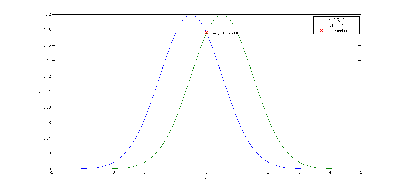

8.在以下条件下重复上机题7：
（a）$p(x|\omega_1) \sim N(-0.5, 2)$及$p(x|\omega_2) \sim N(+0.5, 2)$，$P(\omega_1) = 2/3$及$P(\omega_2) = 1/3$。
（b）$p(x|\omega_1) \sim N(-0.5, 2)$及$p(x|\omega_2) \sim N(+0.5, 2)$，$P(\omega_1) = 1/2$及$P(\omega_2) = 1/2$。
（c）$p(x|\omega_1) \sim N(-0.5, 3)$及$p(x|\omega_2) \sim N(+0.5, 1)$，$P(\omega_1) = 1/2$及$P(\omega_2) = 1/2$。

CH2_8_a.m: Test CH2_7.m with two Gauss distribution.

u1 = -0.5;
sigma1 = 2;
u2 = 0.5;
sigma2 = 2;
P1 = 2/3;
P2 = 1/3;
[Eerror, Bbound, Cerror] = CH2_7(u1, sigma1, u2, sigma2, P1, P2);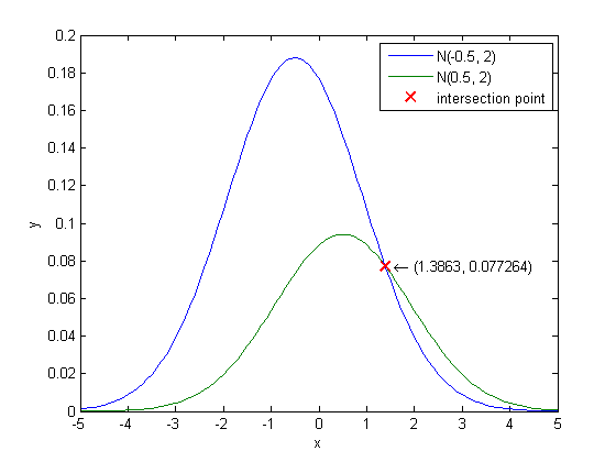

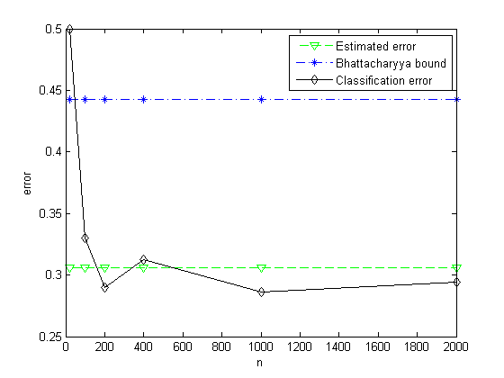
CH2_8_b.m: Test CH2_7.m with two Gauss distribution.

u1 = -0.5;
sigma1 = 2;
u2 = 0.5;
sigma2 = 2;
P1 = 1/2;
P2 = 1/2;
[Eerror, Bbound, Cerror] = CH2_7(u1, sigma1, u2, sigma2, P1, P2);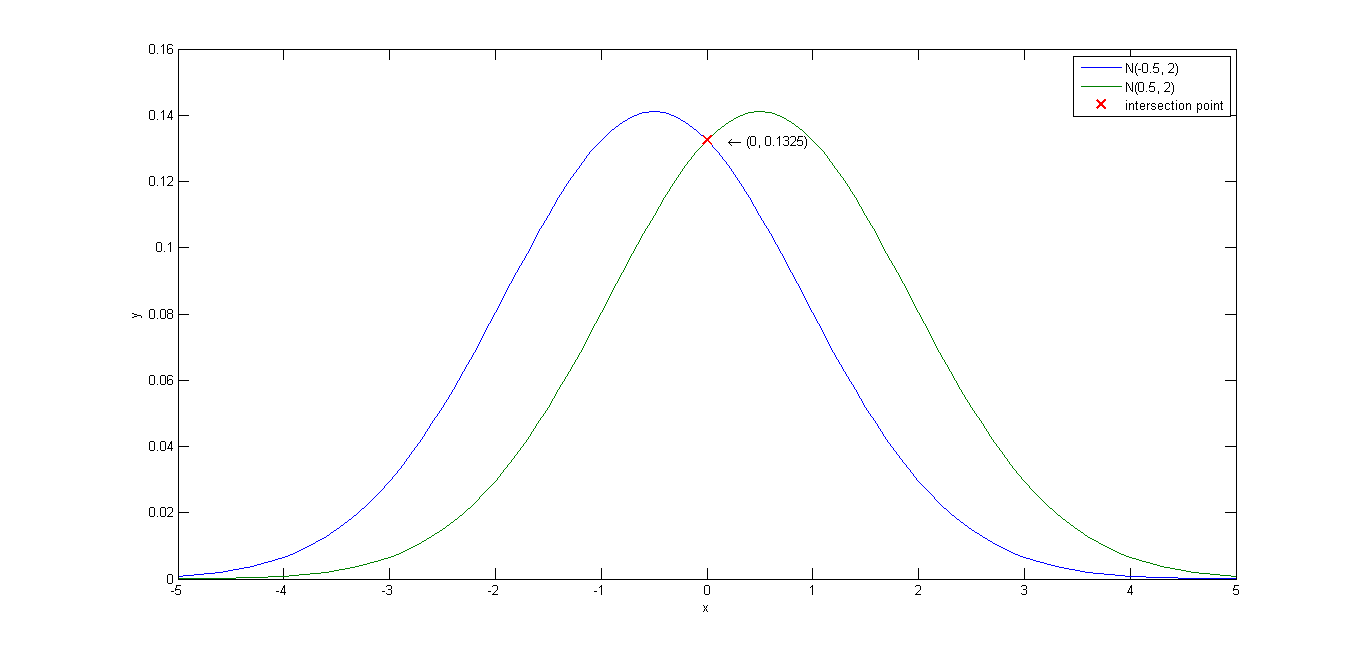

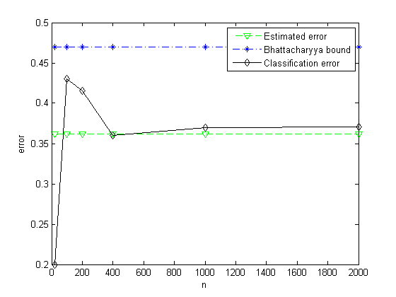
CH2_8_c.m: Test CH2_7.m with two Gauss distribution.

u1 = -0.5;
sigma1 = 3;
u2 = 0.5;
sigma2 = 1;
P1 = 1/2;
P2 = 1/2;
[Eerror, Bbound, Cerror] = CH2_7(u1, sigma1, u2, sigma2, P1, P2);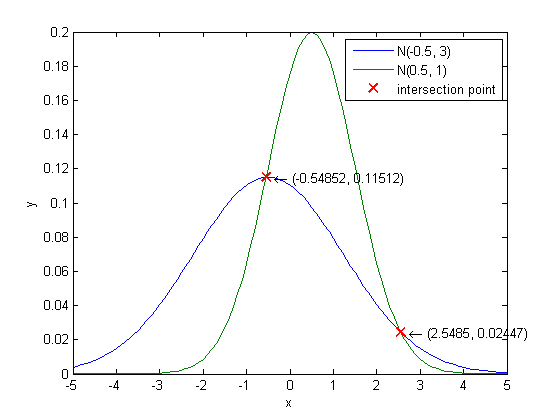

Bhattacharyya.m: Find the Bhattacharyya bound given means and covariances of single gaussian distributions.

function Perror = Bhattacharyya(u1, sigma1, u2, sigma2, P1)
% function Perror = Bhattacharyya(mu1, sigma1, mu2, sigma2, p1)
% Find the Bhattacharyya bound given means and covariances of single
% gaussian distributions.
% Inputs:
%   u1         - Mean of class1
%   sigma1     - Covariance matrix of class1
%   u2         - Mean of class2
%   sigma2     - Covariance matrix of class2
%   P1         - Probability of class1
%
% Outputs
%   Perror      - Error bound

k_half = 1/8*(u2 - u1)'*inv((sigma1 + sigma2)/2)*(u2 - u1) + 1/2*log(det((sigma1+sigma2)/2)/sqrt(det(sigma1)*det(sigma2)));
Perror = sqrt(P1*(1 - P1))*exp(-k_half);

Chernoff.m: Find the Chernoff bound given means and covariances of single gaussian distributions.

function Perror = Chernoff(u1, sigma1, u2, sigma2, P1)
% function Perror = Chernoff(u1, sigma1, u2, sigma2, P1)
% Find the Chernoff bound given means and covariances of single gaussian distributions.
% Inputs:
%   u1         - Mean of class1
%   sigma1     - Covariance matrix of class1
%   u2         - Mean of class2
%   sigma2     - Covariance matrix for class2
%   P1         - Prior probability of class1
%
% Outputs
%   Perror      - Error bound

beta = linspace(0, 1, 100);
k = zeros(1, length(beta));

% calculate k(beta)
for i = 1:length(beta),
    k(i) = beta(i)*(1 - beta(i))/2*(u2 - u1)'*inv(beta(i)*sigma1 + (1 - beta(i))*sigma2)*(u2 - u1) + ...
              1/2*log(det(beta(i)*sigma1 + (1 - beta(i))*sigma2)/(det(sigma1)^beta(i)*det(sigma2)^(1 - beta(i))));
end

% find the minimum of exp(-k)
[m, index] = min(exp(-k));
min_beta = beta(index);

Perror = P1^min_beta*(1 - P1)^(1 - min_beta)*exp(-k(index));
% fprintf('min beta:%f\n', min_beta);
% plot(beta, exp(-k));