


 本文介绍了如何使用PyTorch和TensorFlow计算分类模型的混淆矩阵,详细解释了准确率、精确率、召回率和特异度等评估指标,特别强调了在医学影像等领域的重要性,以及在样本不平衡情况下的模型性能分析。还提供了Python代码实例来创建和解读混淆矩阵图像。
概念
参考视频:
使用pytorch和tensorflow计算分类模型的混淆矩阵_哔哩哔哩_bilibili
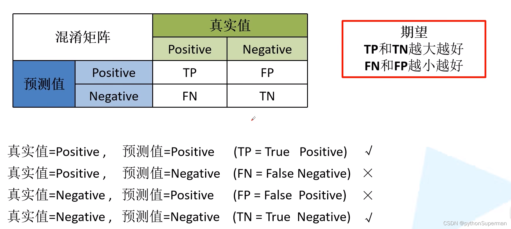
混淆矩阵是评判模型结果的一种指标,属于模型评估的一部分,常用于评判分类器模型的优劣。
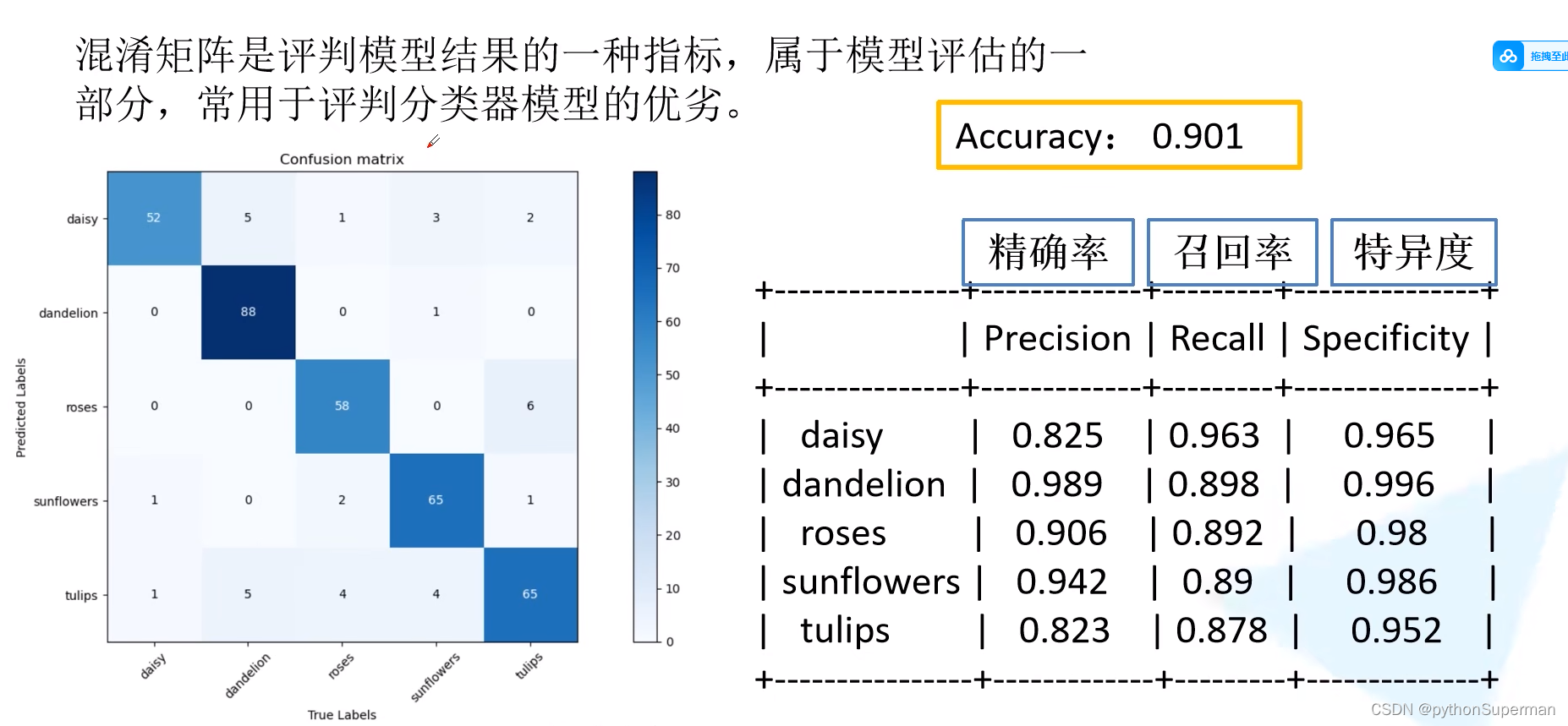
准确率:所有预测正确的验证集样本个数/所有的验证集样本个数。在混淆矩阵中,分子为对角线上所有数字之和,分母为混淆矩阵所有数字之和。
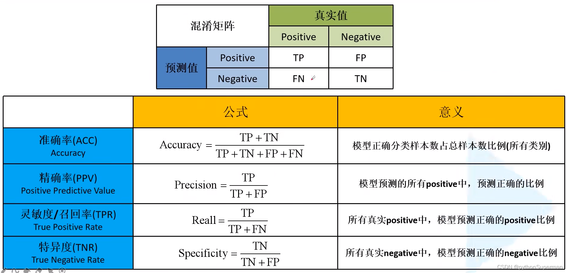
计算公式
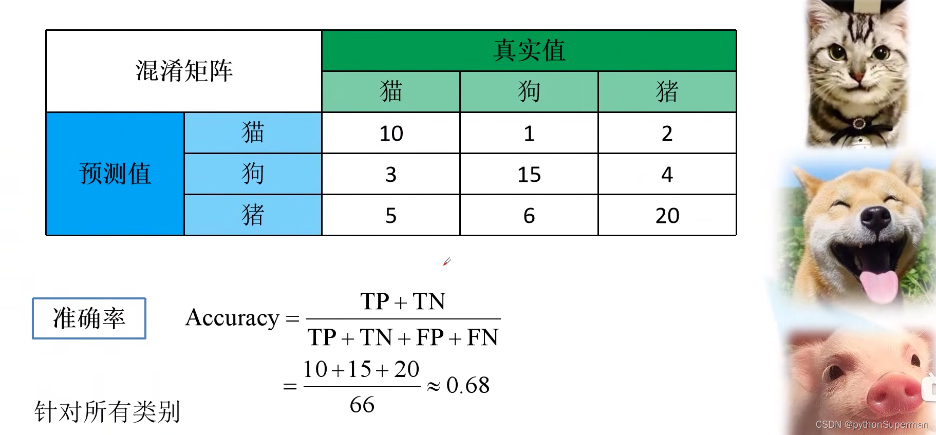
实例
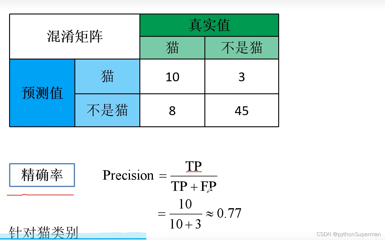
准确率
精确率
召回率(sensitivity)

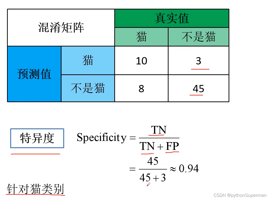
特异度
其他
SE、SP和YI是评估分类模型性能时常用的几个统计指标,特别是在医学影像处理、疾病诊断等领域,这些指标帮助了解模型对于正负类样本的识别能力。
-
SE (Sensitivity),也称为真正率(True Positive Rate, TPR)或召回率(Recall),衡量的是模型正确识别正类(病例)的能力。计算公式为:其中,TP(True Positives)是真正例的数量,FN(False Negatives)是假负例的数量。

-
SP (Specificity),也称为真负率(True Negative Rate, TNR),衡量的是模型正确识别负类(非病例)的能力。计算公式为:其中,TN(True Negatives)是真负例的数量,FP(False Positives)是假正例的数量。

-
YI (Youden’s Index),也称为Youden指数,是一个综合考虑了敏感性和特异性的指标,用于评价测试的总体有效性。计算公式为:Youden指数的范围从0到1,值越大表示测试的性能越好,即同时具有较高的敏感性和特异性。

这些指标对于理解模型在特定任务上的表现至关重要,尤其是在正负样本分布不平衡的情况下。通过评估敏感性和特异性,可以确保模型不仅仅是优先预测多数类,而是真正能够区分不同类别的样本。Youden指数提供了一个简单的度量标准,以确定模型是否在不牺牲一个指标的情况下,同时优化了敏感性和特异性。
代码实战2
import numpy as np
import matplotlib.pyplot as plt
import seaborn as sns
from sklearn.metrics import confusion_matrix
import matplotlib

# 创建示例的混淆矩阵数据
actual_labels = ['cat', 'dog', 'bird']
predicted_labels = ['cat', 'dog', 'bird']
confusion_mat = np.array([[10, 2, 1],
                          [3, 15, 2],
                          [0, 1, 8]])

# 创建混淆矩阵图像
plt.figure(figsize=(8, 6))
sns.heatmap(confusion_mat, annot=True, cmap='Blues', xticklabels=predicted_labels, yticklabels=actual_labels)
# annot=True 参数用于在每个单元格中显示数值  cmap='Blues'参数用于设置颜色映射。

# 添加图像标题和坐标轴标签
plt.title('Confusion Matrix')
plt.xlabel('Predicted Labels')
plt.ylabel('Actual Labels')

# Save the figure
plt.savefig('confusion_matrix.png', dpi=300)  # Saves the plot as a PNG file with 300 DPI

# 显示图像
plt.show()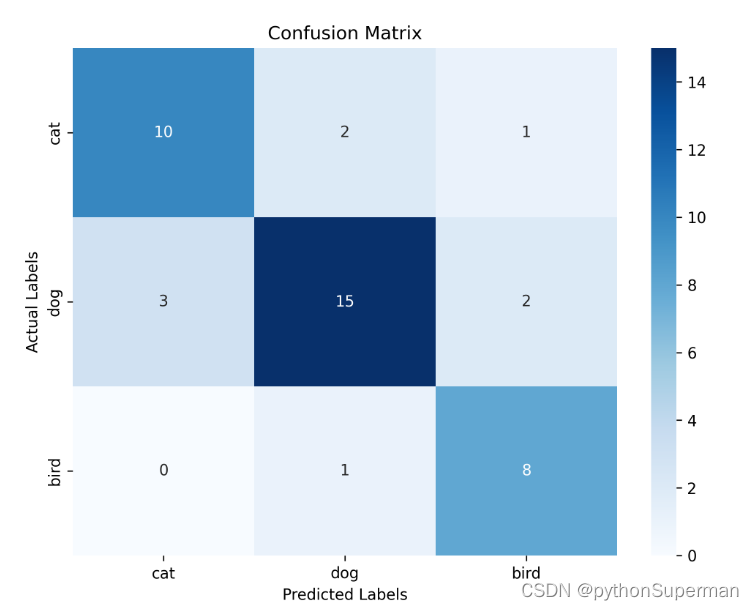
探究每个类的准确率、召回率sensitivity记忆平均准确率的关系
import numpy as np
import matplotlib.pyplot as plt
import seaborn as sns
from sklearn.metrics import confusion_matrix
import matplotlib

# 创建示例的混淆矩阵数据
actual_labels = ['cat', 'dog', 'bird']
predicted_labels = ['cat', 'dog', 'bird']
confusion_mat = np.array([[10, 2, 1],
                          [3, 15, 2],
                          [0, 1, 8]])

# 创建混淆矩阵图像
plt.figure(figsize=(8, 6))
sns.heatmap(confusion_mat, annot=True, cmap='Blues', xticklabels=predicted_labels, yticklabels=actual_labels)
# annot=True 参数用于在每个单元格中显示数值  cmap='Blues'参数用于设置颜色映射。

# 添加图像标题和坐标轴标签
plt.title('Confusion Matrix')
plt.xlabel('Predicted Labels')
plt.ylabel('Actual Labels')

# Save the figure
plt.savefig('confusion_matrix2.png', dpi=300)  # Saves the plot as a PNG file with 300 DPI

# 显示图像
plt.show()

# 计算平均准确率
total_correct = np.trace(confusion_mat)  # 对角线元素之和
total_samples = np.sum(confusion_mat)    # 所有元素之和
average_accuracy = total_correct / total_samples
print(f'Average Accuracy: {average_accuracy:.2f}')

# 计算每个类别的精确度(Precision)
precision_per_class = confusion_mat.diagonal() / np.sum(confusion_mat, axis=0)
for label, precision in zip(actual_labels, precision_per_class):
    print(f'Precision for {label}: {precision:.2f}')

# 计算每个类别的准确率(Recall)
recall_per_class = confusion_mat.diagonal() / np.sum(confusion_mat, axis=1)
for label, recall in zip(actual_labels, recall_per_class):
    print(f'Recall for {label}: {recall:.2f}')
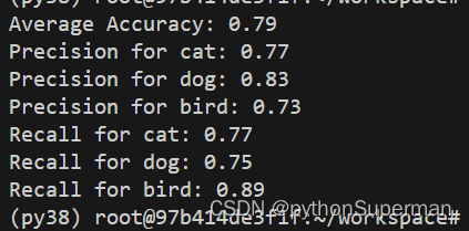
实验结果表明:
每个类的召回率就是每个类的准确率。平均准确率就是就是所有类的召回率的和的平均值。
召回率(Recall)也被称为敏感度(Sensitivity)或真阳性率(True Positive Rate, TPR)
越高的召回率表示模型能够更好地检测出正类样本。


 被折叠的 条评论
为什么被折叠?
被折叠的 条评论
为什么被折叠?
 到【灌水乐园】发言


