


贡献指南
我们非常欢迎您的贡献!如果您有关于新教程的想法或提案,请提交一个 issue并附上大纲。
即使英语不是您的母语,或者您只能提供粗略的草稿,也请不要担心。开源是社区共同努力的结果。尽您所能——我们会帮助解决相关问题。
图片和真实数据能使文本更具吸引力和说服力,但请确保您使用的内容具有适当的许可且可公开使用。同样地,即使只是艺术作品的初步构想,也可以由他人进一步完善。
NumPy 教程是经过精心筛选的 MyST-NB 笔记本集合。这些笔记本用于生成静态网站,也可以通过 Jupytext 在 Jupyter 中作为笔记本打开。
注意: 您应该使用 CommonMark 格式的 markdown 单元格。Jupyter 仅支持渲染 CommonMark。
为什么选择 Jupyter Notebook?
本仓库选用 Jupyter Notebook 而非 NumPy 主文档常用的 reStructuredText 格式,主要基于两个原因:
- Jupyter Notebook 是科学信息交流的通用格式
- 通过 Binder 可直接运行 Jupyter Notebook,方便用户交互式学习教程
- reStructuredText 可能对某些潜在教程贡献者构成技术门槛
注意
您可能会注意到我们的内容采用 Markdown 格式(.md 文件)。我们使用 MyST-NB 格式来审阅和托管笔记本。我们同时接受 Jupyter 笔记本(.ipynb)和 MyST-NB 笔记本(.md)。若需将 .ipynb 文件与 .md 文件同步,请参考 配对教程。
添加自定义教程
如果您拥有自己的 Jupyter notebook 教程文件(.ipynb 格式),并希望将其添加到代码仓库中,请按照以下步骤操作。
创建议题
前往 numpy/numpy-tutorials#issues 并新建一个议题来提交您的提案。请尽可能详细说明您希望撰写的内容类型(教程、操作指南)以及计划涵盖的主题范围。我们将尽快审核并提供反馈意见(如适用)。
查看我们推荐的模板
您可以使用此模板来确保您的内容与现有教程保持一致:
上传你的内容
在上传笔记本文件前,请记得清除所有输出内容。
首先fork这个代码库(如果你之前没有操作过)。

在你的fork仓库中,为你的内容创建一个新分支

将你的笔记本文件添加到content/目录下

更新environment.yml文件
(仅当你添加了新依赖时需要补充相关依赖项)
更新本README.md文件
(将你的新教程条目添加至文档中)

创建一个pull request
请确保勾选"允许维护者编辑和访问机密信息"选项,以便我们顺利审核你的提交内容。

🎉 等待审核!
如需了解更多关于GitHub及其工作流程的信息,请参阅
这份文档
将 Jupyter Notebook 与 MyST-NB 配对使用
你将实现的功能
本指南将保持 Jupyter 笔记本在 .ipynb 和 .md 格式之间同步(或称配对)。
你将学习到
- Jupyter的json格式与MyST-NB的markdown格式之间的区别
- json和markdown格式各自的优缺点
- 如何保持
.ipynb和.md文件同步
准备工作
背景
NumPy 教程以MyST-NB笔记本的形式进行评审和执行。采用Markdown格式更便于审查内容,同时可保持.ipynb文件与NumPy教程内容的同步。NumPy教程使用Jupytext将.ipynb文件转换为MyST Markdown格式。
Jupyter笔记本以JSON格式存储在磁盘上。JSON格式功能强大,可存储Python库生成的几乎所有输入和输出数据。但缺点是评审拉取请求时,难以直观查看和比较笔记本文件的变更,因为评审者只能查看原始JSON文件。
MyST-NB笔记本以Markdown格式存储在磁盘上。Markdown是一种轻量级标记语言,其核心设计目标是可读性。但缺点是Markdown仅能存储代码输入部分,每次打开笔记本时需重新执行输入才能查看输出结果。
注意: 应使用CommonMark标准的Markdown单元。Jupyter仅渲染CommonMark标准的Markdown,而MyST-NB支持多种reStructuredText指令。这些Sphinx Markdown指令在NumPy教程构建为静态网站时会正常渲染,但在本地Jupyter或Binder中打开时会显示为原始代码。
以下为同一个简单笔记本示例的两种版本对比。笔记本包含三个要素:
1、解释代码的Markdown单元
This code calculates 2+2 and prints the output.
2、展示代码的代码单元
x = 2 + 2
print('x = ', x)
3、代码单元的输出
x = 4
简单笔记本示例
这段代码计算2+2并打印输出结果。
x = 2 + 2
print("x = ", x)
x = 4
以下是两个简单笔记本示例的原始输入对比:
json .ipynb
{
 "cells": [
  {
   "cell_type": "markdown",
   "metadata": {},
   "source": [
    "This code calculates 2+2 and prints the output"
   ]
  },
  {
   "cell_type": "code",
   "execution_count": 1,
   "metadata": {},
   "outputs": [
    {
     "name": "stdout",
     "output_type": "stream",
     "text": [
      "x =  4\n"
     ]
    }
   ],
   "source": [
    "x = 2 + 2\n",
    "print('x = ', x)"
   ]
  }
 ],
 "metadata": {
  "kernelspec": {
   "display_name": "Python 3",
   "language": "python",
   "name": "python3"
  },
  "language_info": {
   "codemirror_mode": {
    "name": "ipython",
    "version": 3
   },
   "file_extension": ".py",
   "mimetype": "text/x-python",
   "name": "python",
   "nbconvert_exporter": "python",
   "pygments_lexer": "ipython3",
   "version": "3.8.3"
  }
 },
 "nbformat": 4,
 "nbformat_minor": 4
}
MyST-NB .md
---
jupytext:
  formats: ipynb,md:myst
  text_representation:
    extension: .md
    format_name: myst
    format_version: 0.12
    jupytext_version: 1.6.0
kernelspec:
  display_name: Python 3
  language: python
  name: python3
---

This code calculates 2+2 and prints the output

\```{code-cell} ipython3
x = 2 + 2
print('x = ', x)
\```
The MyST-NB .md is much shorter, but it does not save the output 4.
Pair your notebook files .ipynb and .md
When you submit a Jupyter notebook to NumPy tutorials, we (the reviewers) will convert
it to a MyST-NB format. You can also submit the MyST-NB .md in your
pull request.
To keep the .ipynb and .md in sync–or paired–you need Jupytext.
Install jupytext using:
pip install jupytext
or
conda install jupytext -c conda-forge
Once installed, start your jupyter lab or jupyter notebook
session in the browser. When launching jupyter lab it will ask you to rebuild to include the Jupytext extension.
You can pair the two formats in the classic Jupyter, Jupyter Lab, or the command line:
1、Classic Jupyter Jupytext pairing

2、JupyterLab Jupytext pairing

3、Command line Jupytext pairing
jupytext --set-formats ipynb,myst notebook.ipynb
Then, update either the MyST markdown or notebook file:
jupytext --sync notebook.ipynb
注意: 安装 Jupytext 后,经典的 Jupyter 界面会自动将 MyST 文件作为笔记本打开。在 JupyterLab 中,你可以右键点击并选择“Open With -> Notebook”以笔记本形式打开。代码单元的输出仅会保存在 .ipynb 文件中。
总结
在本教程中,您了解了用于创建 Jupyter Notebook 的 json .ipynb 格式和 MyST-NB .md 原始代码。您可以使用这两种格式来编写教程。现在,您既可以选择在 VIM 或 emacs 这类简易文本编辑器中工作,也可以继续在浏览器中构建 Notebook。Jupytext 能通过配对功能保持您的工作内容同步。
学习编写NumPy教程
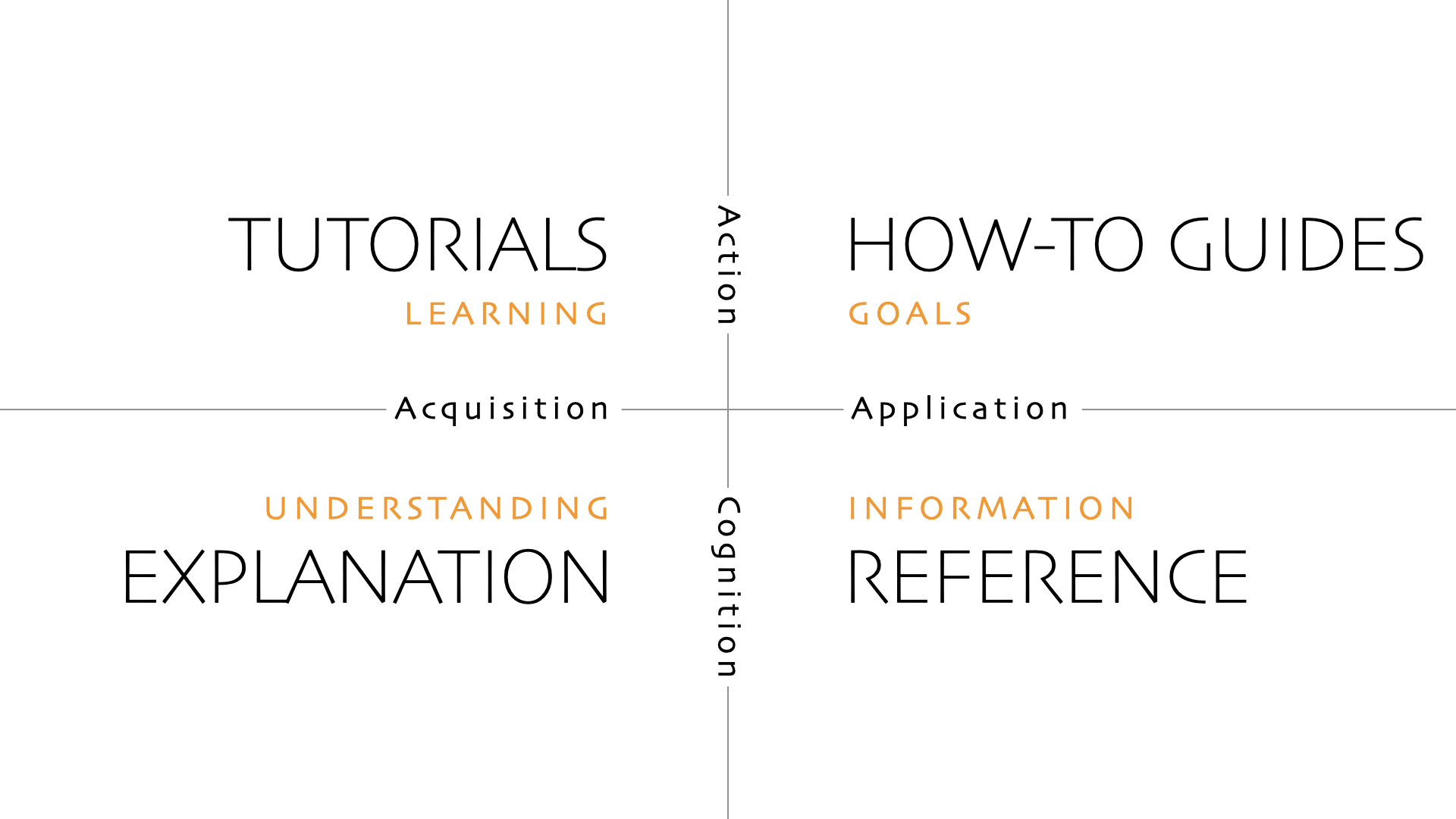
图片来源:Daniele Procida的Diátaxis框架,采用CC-BY-SA 4.0许可协议。
你将完成的任务
根据模板指导,你将编写一篇NumPy教程。
你将学到什么
- 你将能够按照标准格式设计教程,并体现良好的教学实践。
- 你将了解NumPy教程开头的三个标准标题——你将做什么、你将学到什么和你需要准备什么——以及底部可选的一些标题,如自主练习、实际应用和延伸阅读。
- 你将明白你将学到什么与你将做什么之间的区别。
- 你将能够区分教程和操作指南。
- 你将了解不应在你将学到什么部分包含哪些内容。
所需准备
- 本模板
- 目标读者的画像
- 就像学校会列出高阶课程的先修要求一样,你可以假设读者已掌握某些知识(但必须明确列出,如下一条所述)。过度解释会拖慢教程节奏,模糊重点。
- 同时要站在读者角度,思考哪些内容需要沿途解释
- "所需准备"清单应包含:
- 用户开始前需预先安装的软件包(不要列出
numpy这类基础包) - 你在上一条中假设读者已掌握的知识(不要简单写
Python,应具体如熟悉Python迭代器)
- 用户开始前需预先安装的软件包(不要列出
- 轻松热情的语调。想象读者不是坐在台下,而是就在你身旁
- 接受所需准备条目使用不完整句式。无需以"你需要"开头
- 无需英语母语能力。可以寻求他人协助
在水平分割线后开始自定义标题
从这里开始编写您的教程步骤,可以使用任意您选择的标题格式。在教程结束时,请添加另一条水平分割线,并恢复使用标准标题格式。
标题应包含动词
通常来说,标题中需要包含动词。例如,使用学习编写NumPy教程而非"NumPy教程规则"。建议在各级标题中也加入动词。
标题使用小写
首字母大写,之后仅对通常需要大写的单词进行大写(因此不要写成"标题使用小写")。
"你将学到什么"部分应该写什么
避免抽象表述。“关于"是一个提示词:与其写"你将了解NumPy的I/O功能”,不如写成"你将学会如何将逗号分隔的文本文件读入NumPy数组"。
"你将做什么"和"你将学到什么"有何不同?
你将做什么通常用一句话描述最终成果:“你将烘焙一个蛋糕”。这明确了学习终点。你将学到什么则列出多项收获:“你将学会遵循食谱、练习测量食材、掌握判断蛋糕出炉时机的技巧”。
避免旁支内容
正如专业文档作者Daniele Procida所解释的:
不要解释学习者完成教程时不需要了解的内容。
由于教程步骤的设计追求清晰易懂,它们可能达不到生产级标准。是的,你应该分享这些信息,但不是在教程过程中——教程应该保持直接和确定。实践应用部分才是放置细节、例外情况、替代方案等补充说明的合适位置。
使用图表与插图
图表能带来双重好处:既能强化你的观点,又能让页面更具吸引力。与英语能力类似,这里并不要求艺术天赋(或精通绘图工具)。即便你只是扫描一张手绘示意图,后续也有人可以帮你优化完善。
在标题下方添加插图——哪怕仅作装饰用途——也能让你的页面脱颖而出。
尽可能使用真实数据集
读者更容易被真实用例吸引。请确保你拥有该数据的使用权限。
教程与操作指南——相似却不同
教程的读者如同初来乍到的游客,想要了解这个地方的全貌。选择一个具体目标,沿途讲解各个景点。
与操作指南的读者不同(他们清楚自己需要什么),教程读者并不知道自己不了解什么。因此教程需要包含你将完成的任务和你将学到的知识这类标题,而这些标题永远不会出现在操作指南中。
遵循 Google 文档风格指南
NumPy 文档遵循 Google 开发者文档风格指南。该指南不仅解答了常见疑问(例如该用 “crossreference” 还是 “cross-reference”),还包含诸多能提升文档撰写质量的实用建议。
笔记本必须完全可执行
Run all cells 应该执行所有单元格直到文件末尾。如果你要演示一个错误表达式并希望显示回溯信息,请注释该表达式并将回溯内容放入文本单元格中。
(注意,对于包含 <尖括号内文本> 的回溯信息,仅用三个反引号是不够的,必须将尖括号替换为 < 和 >,如下方文本单元格的markdown示例所示。)
# 100/0
--------------------------------------------------------------------------- ZeroDivisionError Traceback (most recent call last) <ipython-input-10-bbe761e74a70> in <module> ----> 1 100/0
ZeroDivisionError: division by zero
自主实践
用一条水平分割线结束教程部分。现在你可以自由选择任何方向,但这里提供三个建议的章节。
在可选的自主实践部分,你可以为读者布置一个练习任务来运用他们新学到的技能。如果是一个有答案的问题,请提供解答——可以用脚注形式呈现,避免直接剧透。
实际应用中…
- 那些被你忽略的细则可以放在这个部分说明。
- 不要仅仅说"通常有其他做法",而要解释原因。
延伸阅读
- 理想情况下,"延伸阅读"部分不应仅提供链接,而应描述参考资料:文档系统是本教程的灵感来源,其中还介绍了其他三种文档类型。
- Google风格指南篇幅较长,这里提供摘要版本。
- NumPy官网包含一份文档编写指南。
文章
帮助改进教程!
想要为教程做出有价值的贡献吗?可以考虑完善以下文章,使其成为完全可执行/可复现的内容!
基于像素输入实现Pong游戏的深度强化学习
注意
由于底层依赖库gym和atari-py存在许可/安装问题,本文当前未经测试。欢迎通过开发依赖更少的示例来改进本文!
本教程演示如何从零实现一个深度强化学习(RL)智能体,使用策略梯度方法,通过NumPy以屏幕像素作为输入来学习玩Pong游戏。您的Pong智能体将使用人工神经网络作为其策略,在游戏过程中实时获取经验。
Pong是1972年推出的一款2D游戏,两名玩家使用"球拍"进行类似乒乓球的对抗。每位玩家通过上下移动屏幕中的球拍,试图击球使其飞向对手方向。游戏目标是让球越过对手球拍使其失球。根据规则,先获得21分的玩家获胜。在本教程中,RL智能体将学习与右侧显示的对手进行对抗。
本示例基于Andrej Karpathy为2017年UC Berkeley举办的深度强化学习训练营开发的代码。他在2016年的博客文章也提供了更多关于Pong RL机制和理论的背景知识。
前提条件
- OpenAI Gym:为了处理游戏环境,您需要使用Gym——这是一个由OpenAI开发的开源Python接口(论文链接),它支持多种模拟环境来帮助完成强化学习任务。
- Python和NumPy:读者需要具备Python基础、NumPy数组操作以及线性代数知识。
- 深度学习和深度强化学习:您应当熟悉深度学习的核心概念,这些概念在Yann LeCun、Yoshua Bengio和Geoffrey Hinton(该领域的先驱者)2015年发表的深度学习论文中有详细阐述。本教程将引导您了解深度强化学习的主要概念,并提供了大量原始文献链接以便参考。
- Jupyter notebook环境:由于强化学习实验可能需要较高的计算资源,您可以通过Binder或Google Colaboratory(提供免费的有限GPU和TPU加速)免费在云端运行本教程。
- Matplotlib:用于绘制图像。请参考安装指南在您的环境中进行配置。
本教程也可以在本地隔离环境中运行,例如Virtualenv和conda。
目录
- 关于强化学习与深度强化学习的说明
- 深度强化学习术语表
1、配置Pong游戏环境
2、帧预处理(观察状态处理)
3、创建策略网络(神经网络)及前向传播
4、设置更新步骤(反向传播)
5、定义折扣奖励函数(预期回报)
6、训练智能体进行3轮游戏
7、后续步骤
8、附录
* 强化学习与深度强化学习笔记
* 如何在Jupyter notebook中设置视频回放功能
关于强化学习与深度强化学习的说明
在强化学习(RL)中,智能体通过所谓的策略与环境交互,通过试错学习获取经验。每次执行动作后,智能体会收到关于奖励(可能获得也可能不获得)以及环境下一观测状态的信息,随后可以继续执行新动作。这一过程会持续多个训练周期,直至任务完成。
智能体的策略工作原理是将观测状态"映射"到对应动作——即根据当前观测状态确定需要执行的动作。总体目标通常是优化智能体的策略,使其在每个观测状态下都能最大化预期奖励。
如需深入了解强化学习,可参考Richard Sutton和Andrew Barton合著的入门书籍。
更多详细信息请查阅本教程末尾的附录部分。
深度强化学习术语表
以下是本教程后续内容中可能用到的深度强化学习术语简明词汇表:
- 在有限时间范围的环境中(如乒乓球游戏),学习智能体可以通过一个回合(episode)来探索(和利用)环境。通常需要多个回合才能使智能体学会策略。
- 智能体通过动作与环境进行交互。
- 执行动作后,智能体会根据所采取的动作和当前所处的状态,通过奖励机制获得反馈(如果有)。状态包含环境的相关信息。
- 智能体的观察值是对状态的部分观测——本教程更倾向于使用这个术语(而非"状态")。
- 智能体可以基于累计奖励(也称为价值函数)和策略来选择动作。累计奖励函数通过智能体的策略来评估其所访问观察值的质量。
- 策略(由神经网络定义)会输出动作选择(以(对数)概率形式),这些选择应该能最大化智能体当前状态的累计奖励。
- 在给定动作条件下,从观察值获得的预期回报称为动作价值函数。为了给短期奖励赋予比长期奖励更大的权重,通常会使用折扣因子(通常是0.9到0.99之间的浮点数)。
- 智能体每次执行策略时的动作和状态(观察值)序列有时被称为轨迹——这样的序列会产生奖励。
您将通过"同策略"方法使用策略梯度来训练乒乓球智能体——这是一种属于基于策略方法家族的算法。策略梯度方法通常使用机器学习中广泛应用的梯度下降来根据长期累计奖励更新策略参数。由于目标是最大化函数(奖励)而非最小化,因此该过程也被称为梯度上升。换句话说,您使用策略让智能体采取动作,目标是通过计算梯度并用它们更新策略(神经)网络中的参数来最大化奖励。
配置Pong游戏环境
1. 首先需要安装OpenAI Gym(通过pip install gym[atari]命令安装——该包目前不提供conda版本),并导入NumPy、Gym以及必要的模块:
import numpy as np
import gym
Gym 可以通过 Monitor 包装器来监控并保存输出:
from gym import wrappers
from gym.wrappers import Monitor
2. 为Pong游戏创建一个Gym环境实例:
env = gym.make("Pong-v0")
3. 让我们来看看 Pong-v0 环境中可用的操作有哪些:
print(env.action_space)
print(env.get_action_meanings())
共有6种动作。但实际上,LEFTFIRE等同于LEFT,RIGHTFIRE对应RIGHT,而NOOP则对应FIRE。
为简化设计,您的策略网络只需输出一个动作——“向上移动”(索引为2或RIGHT)的(对数)概率值。另一个可用动作的索引为3("向下移动"或LEFT)。
4. Gym能够将智能体的学习过程录制为MP4格式视频——通过运行以下代码,用Monitor()包裹环境即可实现:
env = Monitor(env, "./video", force=True)
虽然在Jupyter笔记本中可以执行各种强化学习实验,但要在训练后渲染Gym环境的图像或视频来可视化智能体如何玩Pong游戏可能会相当具有挑战性。如果想在笔记本中设置视频播放功能,可以在本教程末尾的附录中找到详细说明。
预处理帧(观测数据)
在本节中,您将设置一个函数来预处理输入数据(游戏观测帧),使其能够被神经网络消化。神经网络只能处理以浮点类型张量(多维数组)形式存在的输入。
您的智能体将使用Pong游戏的帧(屏幕帧的像素)作为策略网络的输入观测。游戏观测会告诉智能体球的位置信息,然后这些数据将通过前向传递输入到神经网络(策略网络)中。这与DeepMind的DQN方法类似(附录部分会进一步讨论)。
Pong的屏幕帧尺寸为210x160像素,包含3个颜色维度(红、绿、蓝)。这些数组使用uint8(8位整数)编码,观测数据存储在Gym Box实例中。
1. 检查Pong的观测数据:
print(env.observation_space)
在Gym中,智能体的动作和观测可以属于Box(n维空间)或Discrete(固定范围整数)类别。
2、你可以通过以下方式查看随机观测(单帧画面):
1) Setting the random `seed` before initialization (optional).

2) Calling  Gym's `reset()` to reset the environment, which returns an initial observation.

3) Using Matplotlib to display the `render`ed observation.
(有关Gym核心类与方法的更多信息,可参考OpenAI Gym核心API。)
import matplotlib.pyplot as plt

env.seed(42)
env.reset()
random_frame = env.render(mode="rgb_array")
print(random_frame.shape)
plt.imshow(random_frame)
为了将观测数据输入到策略(神经)网络中,需要将其转换为6,400(80x80x1)个浮点数的一维灰度向量。(在训练过程中,可以使用NumPy的np.ravel()函数将这些数组展平。)
3. 设置一个用于帧(观测)预处理的辅助函数:
def frame_preprocessing(observation_frame):
    # Crop the frame.
    observation_frame = observation_frame[35:195]
    # Downsample the frame by a factor of 2、    observation_frame = observation_frame[::2, ::2, 0]
    # Remove the background and apply other enhancements.
    observation_frame[observation_frame == 144] = 0  # Erase the background (type 1).
    observation_frame[observation_frame == 109] = 0  # Erase the background (type 2).
    observation_frame[observation_frame != 0] = 1  # Set the items (rackets, ball) to 1、    # Return the preprocessed frame as a 1D floating-point array.
    return observation_frame.astype(float)
4. 预处理之前随机选取的帧来测试该函数——策略网络的输入是一个80x80的一维图像:
preprocessed_random_frame = frame_preprocessing(random_frame)
plt.imshow(preprocessed_random_frame, cmap="gray")
print(preprocessed_random_frame.shape)
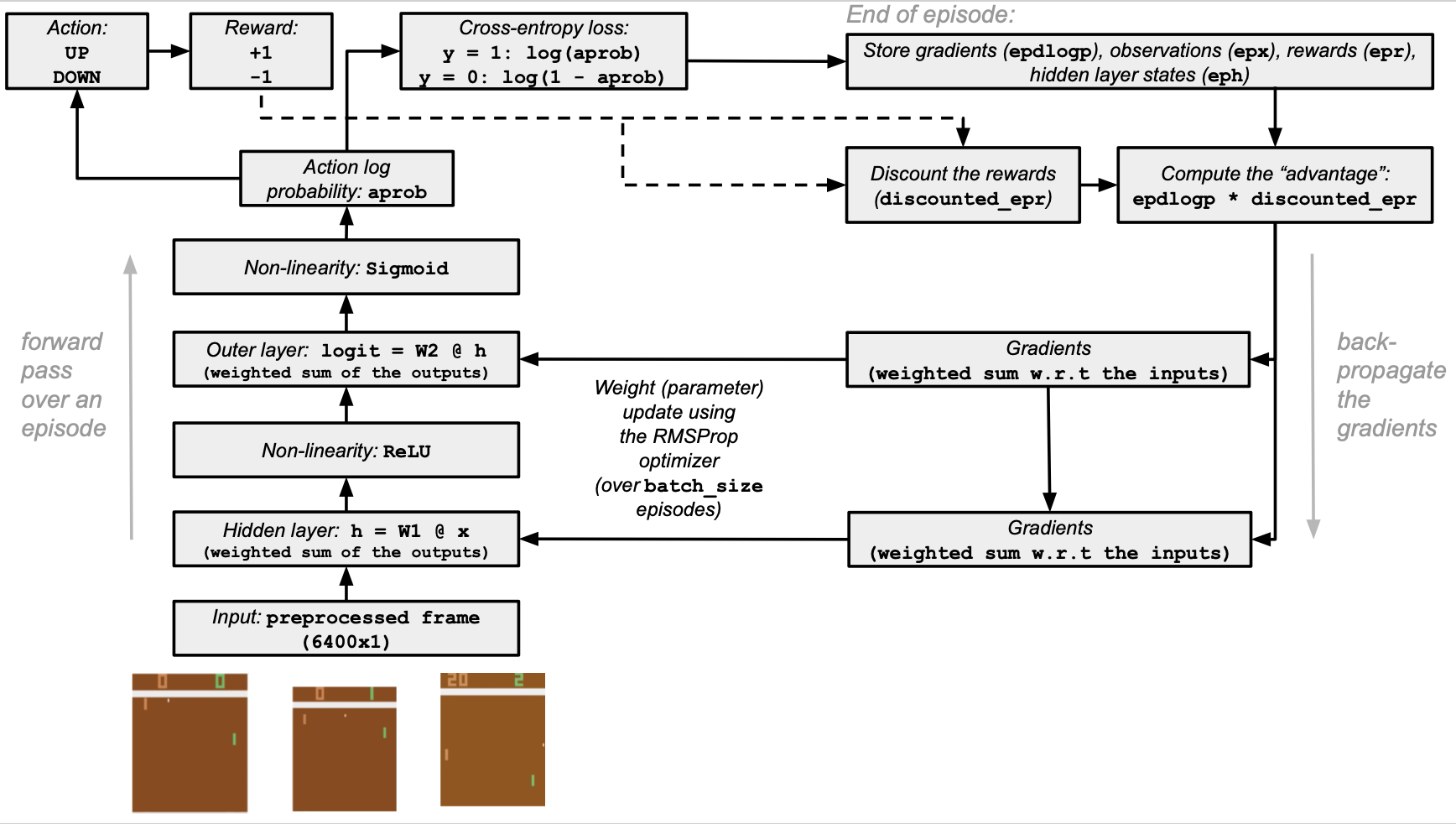
创建策略(神经网络)和前向传播
接下来,我们将策略定义为一个简单的前馈网络,它以游戏观察结果作为输入,输出动作的对数概率:
- 输入层:使用Pong视频游戏帧——预处理后的1D向量,包含6,400个(80x80)浮点数数组。
- 隐藏层:使用NumPy的点积函数
np.dot()计算输入值的加权和,然后应用ReLU等非线性激活函数。 - 输出层:再次执行权重参数与隐藏层输出的矩阵乘法(使用
np.dot()),并通过softmax激活函数传递该信息。 - 最终,策略网络将为智能体输出给定观察状态下某个动作的对数概率——即环境中索引为2的动作(“向上移动球拍”)的概率。
1. 首先为输入层、隐藏层和输出层实例化特定参数,并开始搭建网络模型。
创建一个随机数生成器实例用于实验(设置种子以保证可复现性):
rng = np.random.default_rng(seed=12288743)
然后:
- 设置输入(观测)维度 - 即经过预处理的屏幕帧:
D = 80 * 80
- 设置隐藏层神经元数量
***
H = 200
- 将你的策略(神经网络)网络模型实例化为一个空字典。
model = {}
在神经网络中,权重是重要的可调参数,网络通过数据的前向传播和反向传播来微调这些参数。
2. 使用一种称为Xavier初始化的技术,通过NumPy的Generator.standard_normal()(该函数返回标准正态分布的随机数)以及np.sqrt()来设置网络模型的初始权重。
model["W1"] = rng.standard_normal(size=(H, D)) / np.sqrt(D)
model["W2"] = rng.standard_normal(size=H) / np.sqrt(H)
3. 你的策略网络首先随机初始化权重,并将输入数据(帧)从输入层前馈通过隐藏层传递到输出层。这个过程被称为前向传播,在函数 policy_forward() 中进行了概述:
def policy_forward(x, model):
    # Matrix-multiply the weights by the input in the one and only hidden layer.
    h = np.dot(model["W1"], x)
    # Apply non-linearity with ReLU.
    h[h < 0] = 0
    # Calculate the "dot" product in the outer layer.
    # The input for the sigmoid function is called logit.
    logit = np.dot(model["W2"], h)
    # Apply the sigmoid function (non-linear activation).
    p = sigmoid(logit)
    # Return a log probability for the action 2 ("move up")
    # and the hidden "state" that you need for backpropagation.
    return p, h
请注意,有两种激活函数用于确定输入与输出之间的非线性关系。这些非线性函数会应用于各层的输出:
- 修正线性单元(ReLU):如上文定义为
h[h<0] = 0。它对负输入返回0,对正输入则返回原值。 - Sigmoid函数:如下文定义为
sigmoid()。它会"包裹"最后一层的输出,并返回一个位于(0, 1)范围内的动作对数概率。
4. 使用NumPy的np.exp()单独定义sigmoid函数来计算指数:
def sigmoid(x):
    return 1.0 / (1.0 + np.exp(-x))
设置更新步骤(反向传播)
在深度强化学习算法的训练过程中,你需要使用动作对数概率(给定观察值)和折扣回报(例如在Pong游戏中+1或-1),然后执行反向传递或反向传播来更新参数——即策略网络的权重。
1. 让我们借助NumPy的数组乘法模块来定义反向传递函数(policy_backward()):
np.dot()(矩阵乘法)np.outer()(外积计算)np.ravel()(将数组展平为一维数组)
def policy_backward(eph, epdlogp, model):
    dW2 = np.dot(eph.T, epdlogp).ravel()
    dh = np.outer(epdlogp, model["W2"])
    dh[eph <= 0] = 0
    dW1 = np.dot(dh.T, epx)
    # Return new "optimized" weights for the policy network.
    return {"W1": dW1, "W2": dW2}
利用网络中的中间隐藏"状态"(eph)和动作对数概率的梯度(epdlogp),policy_backward函数将梯度反向传播至策略网络并更新权重。
2. 在智能体训练过程中应用反向传播时,需要为每个回合保存多个变量。我们初始化空列表来存储这些变量:
# All preprocessed observations for the episode.
xs = []
# All hidden "states" (from the network) for the episode.
hs = []
# All gradients of probability actions
# (with respect to observations) for the episode.
dlogps = []
# All rewards for the episode.
drs = []
在训练过程中,当这些变量"填满"后,你需要在每个回合结束时手动重置它们,并使用 NumPy 的 np.vstack() 进行重塑操作。本教程末尾的训练阶段会演示这一过程。
3. 接下来,在优化智能体策略时执行梯度上升操作,通常会使用深度学习优化器(通过梯度进行优化)。本示例将采用 RMSProp——一种自适应优化方法。我们需要为优化器设置一个折扣因子(即衰减率):
decay_rate = 0.99
4. 在训练过程中,你还需要存储梯度(借助 NumPy 的 np.zeros_like())以用于优化步骤:
- 首先,保存那些在批次训练中累积梯度的更新缓冲区:
grad_buffer = {k: np.zeros_like(v) for k, v in model.items()}
- 其次,存储优化器的 RMSProp 内存用于梯度上升:
rmsprop_cache = {k: np.zeros_like(v) for k, v in model.items()}
定义折扣奖励(预期回报)函数
在本节中,您将建立一个用于计算折扣奖励的函数(discount_rewards())——即从某个观察点出发的预期回报。该函数以奖励的一维数组作为输入(借助NumPy的np.zeros_like()函数实现)。
为了给短期奖励赋予比长期奖励更大的权重,您将使用一个折扣因子(gamma),其值通常为0.9至0.99之间的浮点数。
gamma = 0.99

def discount_rewards(r, gamma):
    discounted_r = np.zeros_like(r)
    running_add = 0
    # 从最后一个奖励到第一个...
    for t in reversed(range(0, r.size)):
        # ...重置奖励总和
        if r[t] != 0:
            running_add = 0
        # ...计算折扣奖励
        running_add = running_add * gamma + r[t]

       discounted_r[t] = running_add
    return discounted_r
训练智能体进行多轮游戏
本节介绍如何设置训练过程,在此过程中你的智能体将学习使用其策略来玩Pong游戏。
以下是Pong游戏策略梯度方法的伪代码:
- 实例化策略(即你的神经网络),并随机初始化策略网络中的权重。
- 初始化一个随机观察状态。
- 重复多轮游戏:
- 将观察状态输入策略网络,输出智能体的动作概率(前向传播)。
- 智能体针对每个观察状态采取动作,观察获得的奖励,并收集状态-动作经验轨迹(在预定义的轮数或批次大小范围内)。
- 计算交叉熵(取正值,因为需要最大化奖励而非最小化损失)。
- 对于每批游戏轮次:
- 使用交叉熵计算动作对数概率的梯度。
- 计算累计回报,并使用折扣因子为短期奖励赋予比长期奖励更大的权重。
- 将动作对数概率的梯度乘以折扣后的奖励(即"优势")。
- 执行梯度上升(反向传播)以优化策略网络的参数(其权重)。
- 最大化那些能带来高回报动作的概率。
你可以随时停止训练,或在磁盘上的/video目录中查看保存的游戏MP4视频。你可以根据你的配置设置更合适的最大游戏轮数。
1. 出于演示目的,我们将训练轮数限制为3轮。如果使用硬件加速(CPU和GPU),可以将轮数增加到1,000轮或更多。作为对比,Andrej Karpathy的原始实验大约进行了8,000轮。
max_episodes = 3
2. 设置批次大小和学习率数值:
- 批次大小决定了模型进行参数更新的频率(以回合计)。它表示智能体可以收集状态-动作轨迹的次数。在收集完成后,你可以执行动作概率乘积的最大化操作。
- 学习率有助于限制权重更新的幅度,防止过度修正。
batch_size = 3

learning_rate = 1e-4
3. 为Gym的render方法设置游戏渲染默认变量(该方法用于显示观察结果,属于可选功能但在调试时很有帮助):
render = False
4. 通过调用 reset() 设置智能体的初始(随机)观测状态:
observation = env.reset()
5. 初始化前一个观测值:
prev_x = None
6. 初始化奖励变量和回合计数器:
running_reward = None

reward_sum = 0

episode_number = 0
7. 为了模拟帧间的运动,将策略网络的单一输入帧(x)设置为当前帧与前一预处理帧之间的差值:
def update_input(prev_x, cur_x, D):
    if prev_x is not None:
        x = cur_x - prev_x
    else:
        x = np.zeros(D)
    return x
8. 最后,使用你预定义的函数启动训练循环:
:tags: [output_scroll]

while episode_number < max_episodes:
    # (For rendering.)
    if render:
        env.render()

    # 1、Preprocess the observation (a game frame) and flatten with NumPy's `ravel()`.
    cur_x = frame_preprocessing(observation).ravel()

    # 2、Instantiate the observation for the policy network
    x = update_input(prev_x, cur_x, D)
    prev_x = cur_x

    # 3、Perform the forward pass through the policy network using the observations
    # (preprocessed frames as inputs) and store the action log probabilities
    # and hidden "states" (for backpropagation) during the course of each episode.
    aprob, h = policy_forward(x, model)
    # 4、Let the action indexed at `2` ("move up") be that probability
    # if it's higher than a randomly sampled value
    # or use action `3` ("move down") otherwise.
    action = 2 if rng.uniform() < aprob else 3

    # 5、Cache the observations and hidden "states" (from the network)
    # in separate variables for backpropagation.
    xs.append(x)
    hs.append(h)

    # 6、Compute the gradients of action log probabilities:
    # - If the action was to "move up" (index `2`):
    y = 1 if action == 2 else 0
    # - The cross-entropy:
    # `y*log(aprob) + (1 - y)*log(1-aprob)`
    # or `log(aprob)` if y = 1, else: `log(1 - aprob)`.
    # (Recall: you used the sigmoid function (`1/(1+np.exp(-x)`) to output
    # `aprob` action probabilities.)
    # - Then the gradient: `y - aprob`.
    # 7、Append the gradients of your action log probabilities.
    dlogps.append(y - aprob)
    # 8、Take an action and update the parameters with Gym's `step()`
    # function; obtain a new observation.
    observation, reward, done, info = env.step(action)
    # 9、Update the total sum of rewards.
    reward_sum += reward
    # 10、Append the reward for the previous action.
    drs.append(reward)

    # After an episode is finished:
    if done:
        episode_number += 1
        # 11、Collect and reshape stored values with `np.vstack()` of:
        # - Observation frames (inputs),
        epx = np.vstack(xs)
        # - hidden "states" (from the network),
        eph = np.vstack(hs)
        # - gradients of action log probabilities,
        epdlogp = np.vstack(dlogps)
        # - and received rewards for the past episode.
        epr = np.vstack(drs)

        # 12、Reset the stored variables for the new episode:
        xs = []
        hs = []
        dlogps = []
        drs = []

        # 13、Discount the rewards for the past episode using the helper
        # function you defined earlier...
        discounted_epr = discount_rewards(epr, gamma)
        # ...and normalize them because they have high variance
        # (this is explained below.)
        discounted_epr -= np.mean(discounted_epr)
        discounted_epr /= np.std(discounted_epr)

        # 14、Multiply the discounted rewards by the gradients of the action
        # log probabilities (the "advantage").
        epdlogp *= discounted_epr
        # 15、Use the gradients to perform backpropagation and gradient ascent.
        grad = policy_backward(eph, epdlogp, model)
        # 16、Save the policy gradients in a buffer.
        for k in model:
            grad_buffer[k] += grad[k]
        # 17、Use the RMSProp optimizer to perform the policy network
        # parameter (weight) update at every batch size
        # (by default: every 10 episodes).
        if episode_number % batch_size == 0:
            for k, v in model.items():
                # The gradient.
                g = grad_buffer[k]
                # Use the RMSProp discounting factor.
                rmsprop_cache[k] = (
                    decay_rate * rmsprop_cache[k] + (1 - decay_rate) * g ** 2
                )
                # Update the policy network with a learning rate
                # and the RMSProp optimizer using gradient ascent
                # (hence, there's no negative sign)
                model[k] += learning_rate * g / (np.sqrt(rmsprop_cache[k]) + 1e-5)
                # Reset the gradient buffer at the end.
                grad_buffer[k] = np.zeros_like(v)

        # 18、Measure the total discounted reward.
        running_reward = (
            reward_sum
            if running_reward is None
            else running_reward * 0.99 + reward_sum * 0.01
        )
        print(
            "Resetting the Pong environment. Episode total reward: {} Running mean: {}".format(
                reward_sum, running_reward
            )
        )

        # 19、Set the agent's initial observation by calling Gym's `reset()` function
        # for the next episode and setting the reward sum back to 0、        reward_sum = 0
        observation = env.reset()
        prev_x = None

    # 20、Display the output during training.
    if reward != 0:
        print(
            "Episode {}: Game finished. Reward: {}...".format(episode_number, reward)
            + ("" if reward == -1 else " POSITIVE REWARD!")
        )
几点注意事项:
- 如果你之前运行过实验并想重复执行,
Monitor实例可能仍在运行,这会导致下次训练智能体时抛出错误。因此,你应该先通过调用env.close()来关闭Monitor,方法是取消下方单元格的注释并运行它:
# env.close()
- 在Pong游戏中,如果玩家未能将球击回,则会获得负奖励(-1),而对方玩家则得到+1奖励。由于智能体在Pong游戏中获得的奖励波动较大,最佳实践是使用相同均值(通过
np.mean())和标准差(通过NumPy的np.std())对其进行归一化处理。 - 当仅使用NumPy时,深度强化学习的训练过程(包括反向传播)需要编写多行代码,可能显得较为冗长。这主要是因为未采用带有自动微分库的深度学习框架(这类框架通常能简化此类实验)。本教程将展示如何从零开始实现所有功能,但你也可以使用支持"自动微分"(autodiff)和"自动求导"(autograd)的Python框架——教程末尾会介绍相关内容。
后续步骤
您可能会注意到,如果将训练回合数从100增加到500或1000以上(具体取决于您使用的CPU和GPU硬件),训练强化学习智能体会耗费很长时间。
策略梯度方法在给予足够时间的情况下可以学会任务,但强化学习中的优化本身就是一个具有挑战性的问题。训练智能体学习玩《Pong》或其他任务可能存在样本效率低下的问题,需要大量训练回合。您还可能观察到,即使经过数百回合训练,奖励值仍会出现较大波动。
此外,与许多基于深度学习的算法类似,您需要考虑策略网络需要学习的大量参数。在《Pong》案例中,当网络隐藏层设为200个节点且输入维度为6400(80x80)时,参数量会达到100万甚至更多。因此,增加更多CPU和GPU来辅助训练始终是一个可选项。
您可以使用更先进的基于策略梯度的算法来加速训练、提高参数敏感性并解决其他问题。例如,2017年由John Schulman等人开发的近端策略优化(PPO)这类"自我对抗"方法,曾被用于耗时10个月训练OpenAI Five智能体达到《Dota 2》竞技水平。当然,若将这些方法应用于较小的Gym环境,训练时间应该只需数小时而非数月。
总体而言,强化学习存在诸多挑战和潜在解决方案,您可以通过Matthew Botvinick、Sam Ritter、Jane X. Wang等人在2019年发表的《强化学习的快与慢》了解相关研究进展。
如需深入学习深度强化学习,推荐以下免费资源:
- OpenAI开发的《深度强化学习入门》
- DeepMind和加州大学伯克利分校实践者讲授的深度强化学习课程
- David Silver(DeepMind/UCL)的强化学习课程
虽然使用NumPy从零构建神经网络是学习NumPy和深度学习的绝佳方式,但在实际应用中建议采用专业框架——如PyTorch、JAX、TensorFlow或MXNet。这些框架不仅提供类NumPy API,还内置自动微分和GPU支持,专为高性能数值计算和机器学习设计。
附录
强化学习与深度强化学习要点
- 在监督学习的深度学习任务中(如图像识别、语言翻译或文本分类),通常会使用大量标注数据。然而在强化学习(RL)中,智能体通常不会直接获得明确的正误反馈——它们依赖其他信号(如奖励)来学习。
- 深度强化学习将RL与深度学习相结合。该领域在2013年首次在复杂环境(如视频游戏)中取得重大突破——这比计算机视觉领域的AlexNet突破晚一年。Volodymyr Mnih与DeepMind同事发表的论文《用深度强化学习玩Atari游戏》(2015年更新版)证明,他们训练的智能体能在街机学习环境中以人类水平玩多款经典游戏。其RL算法——深度Q网络(DQN)——在神经网络中使用卷积层来近似Q学习,并采用经验回放技术。
- 与本例使用的简单策略梯度法不同,DQN采用"离策略"的基于价值方法(近似Q学习),而最初的AlphaGo结合了策略梯度和蒙特卡洛树搜索。
- Richard Sutton等人在2000年论述了神经网络等函数近似的策略梯度法。该研究受多项前人工作影响,包括统计梯度跟踪算法如REINFORCE(Ronald Williams,1992)和助力深度学习算法的反向传播(Geoffrey Hinton,1986)。Gerald Tesauro在1990年代的研究中首次将神经网络函数近似引入RL,其1995年论文《时序差分学习与TD-Gammon》记录了1992年与IBM合作开发的双陆棋AI,Long-Ji Lin 1993年也发表了《机器人神经网络的强化学习》。
- 自2013年起,研究者提出了许多用深度RL解决复杂任务的创新方法,包括:围棋AIAlphaGo(David Silver等,2016);通过自我对弈掌握围棋、国际象棋和将棋的AlphaZero(2017-2018);Dota2的OpenAI Five(采用自我对弈,2019);以及星际争霸2的AlphaStar(结合演员-评论家算法、经验回放、自我模仿学习和策略蒸馏,Oriol Vinyals等,2019)。此外还有EA/DICE工程师进行的《战地1》深度RL实验。
- 电子游戏在深度RL研究中广受欢迎的原因之一是:与遥控直升机等现实实验(Pieter Abbeel等,2006)不同,虚拟仿真能提供更安全的测试环境。
- 若想了解深度RL在神经科学等领域的应用,可参考Matthew Botvinick等2020年的论文。
如何在Jupyter笔记本中设置视频播放
- 如果你使用Binder(一个基于Jupyter笔记本的免费工具),可以设置Docker镜像并在
apt.txt配置文件中添加freeglut3-dev、xvfb和x11-utils来安装初始依赖项。接着,在binder/environment.yml的channels下添加gym、pyvirtualdisplay以及其他可能需要的组件,例如python=3.7、pip和jupyterlab。更多信息可参考这篇文章。 - 如果你使用Google Colaboratory(另一个基于Jupyter笔记本的免费工具),可以通过安装并配置X虚拟帧缓冲区/Xvfb、X11、FFmpeg、PyVirtualDisplay、PyOpenGL等依赖项来启用游戏环境的视频播放功能,具体操作如下所述。
1、如果使用Google Colaboratory,请在笔记本单元格中运行以下命令以支持视频播放:
# Install Xvfb and X11 dependencies.
!apt-get install -y xvfb x11-utils > /dev/null 2>&1
# To work with videos, install FFmpeg.
!apt-get install -y ffmpeg > /dev/null 2>&1
# Install PyVirtualDisplay for visual feedback and other libraries/dependencies.
!pip install pyvirtualdisplay PyOpenGL PyOpenGL-accelerate > /dev/null 2>&1
2、然后添加以下Python代码:
# Import the virtual display module.
from pyvirtualdisplay import Display
# Import ipythondisplay and HTML from IPython for image and video rendering.
from IPython import display as ipythondisplay
from IPython.display import HTML

# Initialize the virtual buffer at 400x300 (adjustable size).
# With Xvfb, you should set `visible=False`.
display = Display(visible=False, size=(400, 300))
display.start()

# Check that no display is present.
# If no displays are present, the expected output is `:0`.
!echo $DISPLAY

# Define a helper function to display videos in Jupyter notebooks:.
# (Source: https://star-ai.github.io/Rendering-OpenAi-Gym-in-Colaboratory/)

import sys
import math
import glob
import io
import base64

def show_any_video(mp4video=0):
    mp4list = glob.glob('video/*.mp4')
    if len(mp4list) > 0:
        mp4 = mp4list[mp4video]
        video = io.open(mp4, 'r+b').read()
        encoded = base64.b64encode(video)
        ipythondisplay.display(HTML(data='''<video alt="test" autoplay
                                            loop controls style="height: 400px;">
                                            <source src="data:video/mp4;base64,{0}" type="video/mp4" />
                                            </video>'''.format(encoded.decode('ascii'))))

    else:
        print('Could not find the video!')
如果你想在 Jupyter notebook 中查看最后一段(非常快速的)游戏画面,并且之前已经实现了 show_any_video() 函数,请在单元格中运行以下代码:
show_any_video(-1)
如果你在 Linux 或 macOS 的本地环境中按照本教程操作,可以将大部分代码整合到一个 Python (.py) 文件中。然后,在终端通过 python your-code.py 运行你的 Gym 实验。要启用渲染功能,可以按照 OpenAI Gym 官方文档 使用命令行界面(确保已按照指南安装 Gym 和 Xvfb)。
近十年著名演讲的情感分析
注意:本文目前未经测试。通过使其完全可执行来帮助改进本教程!
本教程演示了如何在NumPy中从头开始构建一个简单的长短期记忆网络(LSTM),用于对社会相关且符合伦理获取的数据集进行情感分析。
您的深度学习模型(LSTM)是循环神经网络的一种形式,将从IMDB影评数据集中学习将文本片段分类为正面或负面。该数据集包含50,000条电影评论及对应标签。基于这些评论的数字表示及其对应标签(监督学习),神经网络将通过时间前向传播和反向传播来学习情感,因为我们在此处理的是序列数据。输出将是一个包含文本样本为正面概率的向量。
如今,深度学习正被应用于日常生活,确保使用AI做出的决策不会对特定人群产生歧视性行为变得尤为重要。在消费AI输出时考虑公平性至关重要。在整个教程中,我们将尝试从伦理角度审视流程中的每个步骤。
前提条件
你需要熟悉 Python 编程语言以及使用 NumPy 进行数组操作。此外,建议具备一定的线性代数和微积分基础。同时,你应当了解神经网络的工作原理。如需参考,可以查阅 Python、n维数组的线性代数 和 微积分 教程。
若需复习深度学习基础知识,建议阅读 d2l.ai 书籍。这是一本结合多框架代码、数学理论和讨论的交互式深度学习教材。你也可以学习 从零实现MNIST深度学习 教程,了解如何从零实现基础神经网络。
除 NumPy 外,本教程将使用以下 Python 标准模块进行数据加载和处理:
pandas用于处理数据框Matplotlib用于数据可视化pooch用于下载和缓存数据集
本教程可在本地隔离环境(如 Virtualenv 或 conda)中运行。你可以使用 Jupyter Notebook 或 JupyterLab 来执行每个笔记本单元。
目录
1、数据收集
2、数据集预处理
3、从头构建并训练LSTM网络
4、对收集的演讲进行情感分析
5、后续步骤
1、数据收集
在开始之前,选择用于训练模型的数据时,请始终牢记以下几点:
- 识别数据偏差 - 偏差是人类思维过程中固有的组成部分。因此,源自人类活动的数据会反映这种偏差。机器学习数据集中常见的偏差类型包括:
- 历史数据偏差:历史数据往往对特定群体存在偏向性或歧视性。数据也可能严重失衡,缺乏对受保护群体的充分记录。
- 数据收集机制偏差:缺乏代表性会导致数据收集过程存在固有偏差。
- 可观测结果偏差:某些情况下,我们仅掌握特定人群的真实结果信息。当缺乏全部结果数据时,甚至无法衡量公平性。
- 敏感数据的人体匿名保护:Trevisan和Reilly列出了需要特别谨慎处理的敏感主题。我们在其基础上补充如下:
- 个人日常活动(包括位置数据);
- 残障详情及/或医疗记录;
- 关于病痛与慢性疾病的情感描述;
- 收入及/或福利支付等财务信息;
- 歧视与虐待事件;
- 对医疗保健和支持服务提供者的批评/赞扬;
- 自杀倾向;
- 可能危及人身安全的对权力结构的批评/赞扬;
- 个人身份信息(即使经过匿名化处理),如指纹或声纹等。
虽然从大量用户(尤其是线上平台)处获取同意可能困难,但其必要性取决于数据涉及的敏感程度,以及数据来源平台是否允许用户使用匿名身份等指标。如果网站强制要求实名制,则必须获得用户明确同意。
本节将收集两个数据集:IMDb电影评论数据集,以及为本教程精选的10篇演讲(涵盖不同国家、时代和主题的 activists)。前者将用于训练深度学习模型,后者将用于情感分析实践。
收集IMDb影评数据集
IMDb影评数据集是由Andrew L. Maas从知名电影评分服务IMDb收集并整理的大型影评数据集。该数据集用于二元情感分类(判断影评属于正面还是负面),包含25,000条训练用影评和25,000条测试用影评。这50,000条带标签数据均可用于监督式深度学习。为确保可复现性,我们将从Zenodo平台获取数据。
IMDb平台允许将其公开数据集用于个人及非商业用途。我们已尽力确保这些影评不包含任何涉及评论者的敏感信息。
收集与加载演讲文本
我们精选了全球活动人士关于气候变化、女权主义、LGBTQA+权益和种族主义等议题的演讲。这些演讲材料来源于报纸、联合国官方网站以及知名大学档案库,具体来源如下表所示。我们创建了一个CSV文件,其中包含转录的演讲内容、演讲者信息以及演讲来源。
在数据收集中,我们确保涵盖不同人群特征,并包含多样化的主题,其中大部分聚焦于社会和/或伦理议题。
| 演讲标题 | 演讲者 | 来源 |
|---|---|---|
| 巴纳德学院毕业典礼演讲 | 莱伊曼·古博薇 | 巴纳德学院 |
| 联合国青年教育演讲 | 马拉拉·优素福扎伊 | 卫报 |
| 联合国大会种族歧视问题讲话 | 琳达·托马斯-格林菲尔德 | 美国驻联合国代表团 |
| 你们怎敢 | 格蕾塔·通贝里 | NBC新闻 |
| 让世界沉默五分钟的演讲 | 瑟玟·铃木 | 地球宪章 |
| 希望演讲 | 哈维·米尔克 | 波士顿美术博物馆 |
| "茁壮成长"大会演讲 | 艾伦·佩吉 | 赫芬顿邮报 |
| 我有一个梦想 | 马丁·路德·金 | 马歇尔大学 |
2、预处理数据集
在构建任何深度学习模型之前,数据预处理都是极其关键的一步。但为了使本教程聚焦于模型构建,我们将不深入探讨预处理代码的细节。以下简要概述了我们为清洗数据并转换为数值表示所采取的所有步骤。
1、文本去噪:在将文本转换为向量之前,必须对其进行清理,去除所有无用的部分(即噪声),包括将所有字符转换为小写、删除HTML标签、括号以及停用词(对句子意义贡献不大的词)。若不进行此步骤,数据集通常会成为计算机无法理解的杂乱词堆。
2、将词语转换为向量:词嵌入是一种学习得到的文本表示方法,具有相同含义的词语会获得相似的表示。单个词被表示为预定义向量空间中的实值向量。GloVe是斯坦福大学开发的一种无监督算法,通过从语料库生成全局词-词共现矩阵来生成词嵌入。您可以从https://nlp.stanford.edu/projects/glove/下载包含嵌入的压缩文件。这里有四种不同大小或训练数据集的选项可供选择。我们选择了内存消耗最少的嵌入文件。
GloVe词嵌入包含基于数十亿甚至高达8400亿标记训练得到的集合。这些算法会表现出刻板偏见,例如可追溯到原始训练数据的性别偏见。例如,某些职业似乎更偏向特定性别,强化了有问题的刻板印象。目前最接近的解决方案是一些去偏算法,如https://web.stanford.edu/class/archive/cs/cs224n/cs224n.1184/reports/6835575.pdf中提出的方法,用户可将其应用于所选嵌入以减少偏见(如果存在)。
接下来,您需要导入构建深度学习网络所需的必要包。
# Importing the necessary packages
import numpy as np
import pandas as pd
import matplotlib.pyplot as plt
import pooch
import string
import re
import zipfile
import os

# Creating the random instance
rng = np.random.default_rng()
接下来,你将定义一组文本预处理辅助函数。
class TextPreprocess:
    """Text Preprocessing for a Natural Language Processing model."""

    def txt_to_df(self, file):
        """Function to convert a txt file to pandas dataframe.

        Parameters
        ----------
        file : str
            Path to the txt file.

        Returns
        -------
        Pandas dataframe
            txt file converted to a dataframe.

        """
        with open(imdb_train, 'r') as in_file:
            stripped = (line.strip() for line in in_file)
            reviews = {}
            for line in stripped:
                lines = [splits for splits in line.split("\t") if splits != ""]
                reviews[lines[1]] = float(lines[0])

       df = pd.DataFrame(reviews.items(), columns=['review', 'sentiment'])

       df = df.sample(frac=1).reset_index(drop=True)
        return df

    def unzipper(self, zipped, to_extract):
        """Function to extract a file from a zipped folder.

        Parameters
        ----------
        zipped : str
            Path to the zipped folder.

        to_extract: str
            Path to the file to be extracted from the zipped folder

        Returns
        -------
        str
            Path to the extracted file.

        """
        fh = open(zipped, 'rb')
        z = zipfile.ZipFile(fh)
        outdir = os.path.split(zipped)[0]
        z.extract(to_extract, outdir)
        fh.close()
        output_file = os.path.join(outdir, to_extract)
        return output_file

    def cleantext(self, df, text_column=None,
                   remove_stopwords=True, remove_punc=True):
        """Function to clean text data.

        Parameters
        ----------

       df : pandas dataframe
            The dataframe housing the input data.
        text_column : str
            Column in dataframe whose text is to be cleaned.
        remove_stopwords : bool
            if True, remove stopwords from text
        remove_punc : bool
            if True, remove punctuation symbols from text

        Returns
        -------
        Numpy array
            Cleaned text.

        """
        # converting all characters to lowercase

       df[text_column] = df[text_column].str.lower()

        # List of stopwords taken from https://gist.github.com/sebleier/554280
        stopwords = ["a", "about", "above", "after", "again", "against",
                      "all", "am", "an", "and", "any", "are",
                      "as", "at", "be", "because",
                      "been", "before", "being", "below",
                      "between", "both", "but", "by", "could",
                      "did", "do", "does", "doing", "down", "during",
                      "each", "few", "for", "from", "further",
                      "had", "has", "have", "having", "he",
                      "he'd", "he'll", "he's", "her", "here",
                      "here's", "hers", "herself", "him",
                      "himself", "his", "how", "how's", "i",
                      "i'd", "i'll", "i'm", "i've",
                      "if", "in", "into",
                      "is", "it", "it's", "its",
                      "itself", "let's", "me", "more",
                      "most", "my", "myself", "nor", "of",
                      "on", "once", "only", "or",
                      "other", "ought", "our", "ours",
                      "ourselves", "out", "over", "own", "same",
                      "she", "she'd", "she'll", "she's", "should",
                      "so", "some", "such", "than", "that",
                      "that's", "the", "their", "theirs", "them",
                      "themselves", "then", "there", "there's",
                      "these", "they", "they'd", "they'll",
                      "they're", "they've", "this", "those",
                      "through", "to", "too", "under", "until", "up",
                      "very", "was", "we", "we'd", "we'll",
                      "we're", "we've", "were", "what",
                      "what's", "when", "when's",
                      "where", "where's",
                      "which", "while", "who", "who's",
                      "whom", "why", "why's", "with",
                      "would", "you", "you'd", "you'll",
                      "you're", "you've",
                      "your", "yours", "yourself", "yourselves"]


       def remove_stopwords(data, column):

       data[f'{column} without stopwords'] = data[column].apply(
                lambda x: ' '.join([word for word in x.split() if word not in (stopwords)]))
            return data


       def remove_tags(string):
            result = re.sub('<*>', '', string)
            return result

        # remove html tags and brackets from text
        if remove_stopwords:

       data_without_stopwords = remove_stopwords(df, text_column)

       data_without_stopwords[f'clean_{text_column}'] = data_without_stopwords[f'{text_column} without stopwords'].apply(
                lambda cw: remove_tags(cw))
        if remove_punc:

       data_without_stopwords[f'clean_{text_column}'] = data_without_stopwords[f'clean_{text_column}'].str.replace(

           '[{}]'.format(string.punctuation), ' ', regex=True)

        X = data_without_stopwords[f'clean_{text_column}'].to_numpy()

        return X

    def sent_tokeniser(self, x):
        """Function to split text into sentences.

        Parameters
        ----------
        x : str
            piece of text

        Returns
        -------
        list
            sentences with punctuation removed.

        """
        sentences = re.split(r'(?<!\w.\w.)(?<![A-Z][a-z].)(?<=.|\?)\s', x)
        sentences.pop()
        sentences_cleaned = [re.sub(r'[^\w\s]', '', x) for x in sentences]
        return sentences_cleaned

    def word_tokeniser(self, text):
        """Function to split text into tokens.

        Parameters
        ----------
        x : str
            piece of text

        Returns
        -------
        list
            words with punctuation removed.

        """
        tokens = re.split(r"([-\s.,;!?])+", text)
        words = [x for x in tokens if (
            x not in '- \t\n.,;!?\\' and '\\' not in x)]
        return words

    def loadGloveModel(self, emb_path):
        """Function to read from the word embedding file.

        Returns
        -------

       dict
            mapping from word to corresponding word embedding.

        """
        print("Loading Glove Model")
        File = emb_path
        f = open(File, 'r')
        gloveModel = {}
        for line in f:
            splitLines = line.split()
            word = splitLines[0]
            wordEmbedding = np.array([float(value) for value in splitLines[1:]])
            gloveModel[word] = wordEmbedding
        print(len(gloveModel), " words loaded!")
        return gloveModel

    def text_to_paras(self, text, para_len):
        """Function to split text into paragraphs.

        Parameters
        ----------
        text : str
            piece of text

        para_len : int
            length of each paragraph

        Returns
        -------
        list
            paragraphs of specified length.

        """
        # split the speech into a list of words
        words = text.split()
        # obtain the total number of paragraphs
        no_paras = int(np.ceil(len(words)/para_len))
        # split the speech into a list of sentences
        sentences = self.sent_tokeniser(text)
        # aggregate the sentences into paragraphs
        k, m = divmod(len(sentences), no_paras)
        agg_sentences = [sentences[i*k+min(i, m):(i+1)*k+min(i+1, m)] for i in range(no_paras)]
        paras = np.array([' '.join(sents) for sents in agg_sentences])

        return paras
Pooch 是一个由科学家开发的 Python 包,用于管理通过 HTTP 下载数据文件并将其存储在本地目录中。我们利用它来建立一个下载管理器,该管理器包含从我们的注册表中获取数据文件所需的所有信息,并将它们存储在指定的缓存文件夹中。
data = pooch.create(
    # folder where the data will be stored in the     # default cache folder of your Operating System
    path=pooch.os_cache("numpy-nlp-tutorial"),    # Base URL of the remote data store
    base_url="",    # The cache file registry. A dictionary with all files managed by this pooch.
    # The keys are the file names and values are their respective hash codes which
    # ensure we download the same, uncorrupted file each time.
    registry={
        "imdb_train.txt": "6a38ea6ab5e1902cc03f6b9294ceea5e8ab985af991f35bcabd301a08ea5b3f0", "imdb_test.txt": "7363ef08ad996bf4233b115008d6d7f9814b7cc0f4d13ab570b938701eadefeb", "glove.6B.50d.zip": "617afb2fe6cbd085c235baf7a465b96f4112bd7f7ccb2b2cbd649fed9cbcf2fb",    },    # Now specify custom URLs for some of the files in the registry.
    urls={
        "imdb_train.txt": "doi:10.5281/zenodo.4117827/imdb_train.txt", "imdb_test.txt": "doi:10.5281/zenodo.4117827/imdb_test.txt", "glove.6B.50d.zip": 'https://nlp.stanford.edu/data/glove.6B.zip'
    }
)
下载IMDb训练和测试数据文件:
imdb_train = data.fetch('imdb_train.txt')
imdb_test = data.fetch('imdb_test.txt')
实例化 TextPreprocess 类以对数据集执行多种操作:
textproc = TextPreprocess()
将每个IMDb文件转换为pandas数据框,以便更方便地对数据集进行预处理:
train_df = textproc.txt_to_df(imdb_train)
test_df = textproc.txt_to_df(imdb_test)
现在,你需要通过去除停用词和标点符号来清理上面得到的数据框。同时,你还需要从每个数据框中提取情感值,以获取目标变量:
X_train = textproc.cleantext(train_df,
                        text_column='review',
                        remove_stopwords=True,
                        remove_punc=True)[0:2000]

X_test = textproc.cleantext(test_df,
                        text_column='review',
                        remove_stopwords=True,
                        remove_punc=True)[0:1000]

y_train = train_df['sentiment'].to_numpy()[0:2000]
y_test = test_df['sentiment'].to_numpy()[0:1000]
同样的处理流程也适用于收集到的演讲文本:
由于后续教程中我们将对每篇演讲进行逐段情感分析,需要借助标点符号将文本分割成段落,因此现阶段我们暂不删除这些标点符号。
speech_data_path = 'tutorial-nlp-from-scratch/speeches.csv'
speech_df = pd.read_csv(speech_data_path)
X_pred = textproc.cleantext(speech_df,
                             text_column='speech',
                             remove_stopwords=True,
                             remove_punc=False)
speakers = speech_df['speaker'].to_numpy()
现在你将下载 GloVe 词向量,解压后构建一个字典来映射每个单词及其对应的词向量。这将作为缓存使用,以便在需要时将每个单词替换为其相应的词向量。
glove = data.fetch('glove.6B.50d.zip')
emb_path = textproc.unzipper(glove, 'glove.6B.300d.txt')
emb_matrix = textproc.loadGloveModel(emb_path)
3、构建深度学习模型
现在开始实现我们的LSTM模型!首先需要熟悉深度学习模型基本构建模块的一些高层概念。可以参考从零开始的MNIST深度学习教程来了解相关内容。
接下来将学习循环神经网络(RNN)与普通神经网络的区别,以及为什么RNN特别适合处理序列数据。之后,你将用Python和NumPy构建一个简单深度学习模型的组件模块,并训练该模型以一定准确率学会判断文本片段的情感倾向(正面或负面)。
长短期记忆网络简介
在多层感知机(MLP)中,信息仅单向流动——从输入层经过隐藏层到达输出层。信息直接穿过网络,后续阶段从不考虑先前的节点。由于它只考虑当前输入,所学习到的特征不会在序列的不同位置间共享。此外,它无法处理长度可变的序列。
与MLP不同,循环神经网络(RNN)专为序列预测问题设计。RNN通过引入状态变量来存储过去的信息,结合当前输入以确定当前输出。由于RNN将学习到的特征与序列中所有数据点共享(无论序列长度如何),因此能够处理可变长度的序列。
然而RNN的问题是:它无法保持长期记忆,因为给定输入对隐藏层(进而对网络输出)的影响会在循环连接中呈指数级衰减或爆炸。这一缺陷被称为梯度消失问题。长短期记忆网络(LSTM)是一种专门为解决梯度消失问题而设计的RNN架构。
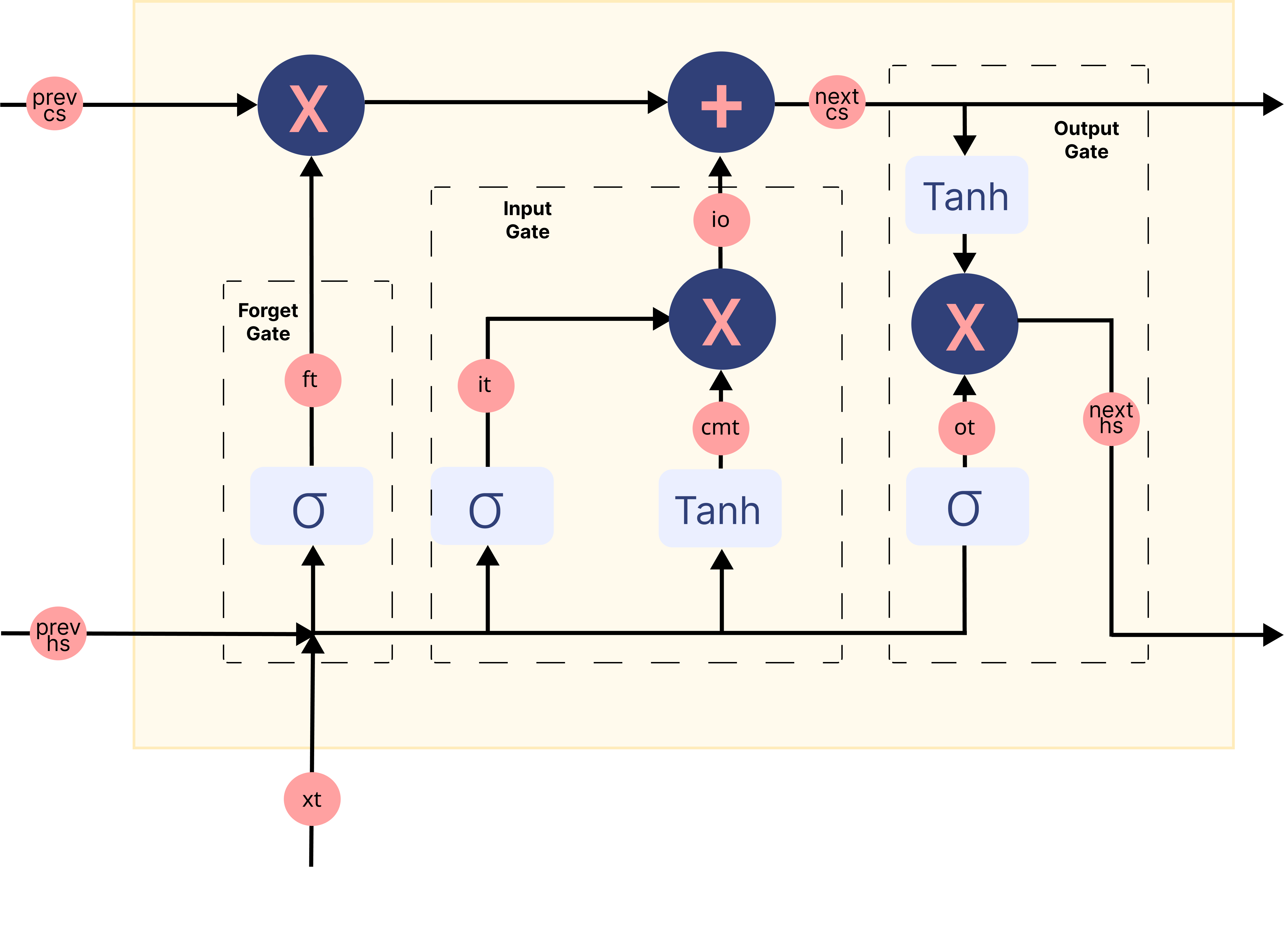
模型架构概述
在上面的动图中,标记为\(A)的矩形称为单元(Cells),它们是我们LSTM网络的记忆块(Memory Blocks)。这些单元负责决定在序列中记住哪些信息,并通过两种状态——隐藏状态(hidden state) \(H_{t})和单元状态(cell state) \(C_{t})(其中\(t)表示时间步长)——将这些信息传递给下一个单元。每个单元都配有专用门控机制,负责存储、写入或读取传递给LSTM的信息。接下来我们将通过实现网络内部的每个机制来详细研究其架构。
首先,我们编写一个函数来随机初始化模型训练过程中需要学习的参数。
def initialise_params(hidden_dim, input_dim):
    # forget gate
    Wf = rng.standard_normal(size=(hidden_dim, hidden_dim + input_dim))
    bf = rng.standard_normal(size=(hidden_dim, 1))
    # input gate
    Wi = rng.standard_normal(size=(hidden_dim, hidden_dim + input_dim))
    bi = rng.standard_normal(size=(hidden_dim, 1))
    # candidate memory gate
    Wcm = rng.standard_normal(size=(hidden_dim, hidden_dim + input_dim))
    bcm = rng.standard_normal(size=(hidden_dim, 1))
    # output gate
    Wo = rng.standard_normal(size=(hidden_dim, hidden_dim + input_dim))
    bo = rng.standard_normal(size=(hidden_dim, 1))

    # fully connected layer for classification
    W2 = rng.standard_normal(size=(1, hidden_dim))
    b2 = np.zeros((1, 1))

    parameters = {
        "Wf": Wf, "bf": bf, "Wi": Wi, "bi": bi, "Wcm": Wcm, "bcm": bcm, "Wo": Wo, "bo": bo, "W2": W2, "b2": b2
    }
    return parameters
前向传播
初始化参数后,您可以将输入数据沿网络正向传递。每一层接收输入数据,处理后传递给下一层,这一过程称为前向传播。具体实现步骤如下:
- 加载输入数据的词嵌入向量
- 将嵌入向量输入LSTM层
- 在LSTM的每个记忆单元中执行所有门控机制,获取最终隐藏状态
- 将最终隐藏状态通过全连接层,得到序列为正例的概率
- 将所有计算值存入缓存,供反向传播时使用
Sigmoid属于非线性激活函数家族。它帮助网络决定更新或遗忘数据:当函数输出为0时信息被遗忘,输出为1时则保留信息。
def sigmoid(x):
    n = np.exp(np.fmin(x, 0))
    d = (1 + np.exp(-np.abs(x)))
    return n / d
遗忘门将当前词嵌入向量与前一隐藏状态拼接后作为输入,决定旧记忆单元内容中哪些部分需要关注、哪些可以忽略。
def fp_forget_gate(concat, parameters):
    ft = sigmoid(np.dot(parameters['Wf'], concat)
                 + parameters['bf'])
    return ft
输入门将当前词嵌入向量与前一隐藏状态拼接后作为输入,并通过候选记忆门控制新数据的纳入程度。候选记忆门利用Tanh函数来调节网络中流动的数值。
def fp_input_gate(concat, parameters):
    it = sigmoid(np.dot(parameters['Wi'], concat)
                 + parameters['bi'])
    cmt = np.tanh(np.dot(parameters['Wcm'], concat)
                  + parameters['bcm'])
    return it, cmt
最终我们来看输出门,它接收来自当前词嵌入、前一个隐藏状态的信息,以及经过遗忘门和输入门信息更新后的细胞状态,用于更新隐藏状态的值。
def fp_output_gate(concat, next_cs, parameters):
    ot = sigmoid(np.dot(parameters['Wo'], concat)
                 + parameters['bo'])
    next_hs = ot * np.tanh(next_cs)
    return ot, next_hs
下图总结了LSTM网络记忆块中每个门控机制的工作原理:
图片修改自此来源
但如何从LSTM的输出中获取情感信息?
从序列中最后一个记忆块的输出门获得的隐藏状态,被视为包含该序列所有信息的表征。为了将这些信息分类到不同类别(本例中为2类:正面和负面),我们使用全连接层,首先将这些信息映射到预定义的输出尺寸(本例中为1)。然后,通过sigmoid等激活函数将此输出转换为0到1之间的值。我们将大于0.5的值视为具有正面情感倾向。
def fp_fc_layer(last_hs, parameters):
    z2 = (np.dot(parameters['W2'], last_hs)
          + parameters['b2'])
    a2 = sigmoid(z2)
    return a2
现在,你需要将这些函数整合起来,总结出我们模型架构中的前向传播步骤:
def forward_prop(X_vec, parameters, input_dim):

    hidden_dim = parameters['Wf'].shape[0]
    time_steps = len(X_vec)

    # Initialise hidden and cell state before passing to first time step
    prev_hs = np.zeros((hidden_dim, 1))
    prev_cs = np.zeros(prev_hs.shape)

    # Store all the intermediate and final values here
    caches = {'lstm_values': [], 'fc_values': []}

    # Hidden state from the last cell in the LSTM layer is calculated.
    for t in range(time_steps):
        # Retrieve word corresponding to current time step
        x = X_vec[t]
        # Retrieve the embedding for the word and reshape it to make the LSTM happy
        xt = emb_matrix.get(x, rng.random(size=(input_dim, 1)))
        xt = xt.reshape((input_dim, 1))

        # Input to the gates is concatenated previous hidden state and current word embedding
        concat = np.vstack((prev_hs, xt))

        # Calculate output of the forget gate
        ft = fp_forget_gate(concat, parameters)

        # Calculate output of the input gate
        it, cmt = fp_input_gate(concat, parameters)
        io = it * cmt

        # Update the cell state
        next_cs = (ft * prev_cs) + io

        # Calculate output of the output gate
        ot, next_hs = fp_output_gate(concat, next_cs, parameters)

        # store all the values used and calculated by
        # the LSTM in a cache for backward propagation.
        lstm_cache = {
        "next_hs": next_hs, "next_cs": next_cs, "prev_hs": prev_hs, "prev_cs": prev_cs, "ft": ft, "it" : it, "cmt": cmt, "ot": ot, "xt": xt, }
        caches['lstm_values'].append(lstm_cache)

        # Pass the updated hidden state and cell state to the next time step
        prev_hs = next_hs
        prev_cs = next_cs

    # Pass the LSTM output through a fully connected layer to     # obtain probability of the sequence being positive
    a2 = fp_fc_layer(next_hs, parameters)

    # store all the values used and calculated by the     # fully connected layer in a cache for backward propagation.
    fc_cache = {
    "a2" : a2,    "W2" : parameters['W2']
    }
    caches['fc_values'].append(fc_cache)
    return caches
反向传播
在每次前向传播完成后,需要实现随时间反向传播算法来累积每个参数随时间步长的梯度。由于LSTM底层层的特殊交互方式,其反向传播过程不像其他常见深度学习架构那样直接。但核心方法基本相同:识别依赖关系并应用链式法则。
首先定义一个函数,将每个参数的梯度初始化为与对应参数维度相同的零数组。
# Initialise the gradients
def initialize_grads(parameters):
    grads = {}
    for param in parameters.keys():
        grads[f'd{param}'] = np.zeros((parameters[param].shape))
    return grads
现在,我们为每个门控单元和全连接层定义一个函数,用于计算损失相对于输入数据和所用参数的梯度。要理解这些导数计算背后的数学原理,我们建议您参考Christina Kouridi撰写的这篇实用博客。
定义遗忘门的梯度计算函数:
def bp_forget_gate(hidden_dim, concat, dh_prev, dc_prev, cache, gradients, parameters):
    # dft = dL/da2 * da2/dZ2 * dZ2/dh_prev * dh_prev/dc_prev * dc_prev/dft
    dft = ((dc_prev * cache["prev_cs"] + cache["ot"]
           * (1 - np.square(np.tanh(cache["next_cs"])))
           * cache["prev_cs"] * dh_prev) * cache["ft"] * (1 - cache["ft"]))
    # dWf = dft * dft/dWf
    gradients['dWf'] += np.dot(dft, concat.T)
    # dbf = dft * dft/dbf
    gradients['dbf'] += np.sum(dft, axis=1, keepdims=True)
    # dh_f = dft * dft/dh_prev
    dh_f = np.dot(parameters["Wf"][:, :hidden_dim].T, dft)
    return dh_f, gradients
定义一个函数来计算输入门和候选记忆门中的梯度:
def bp_input_gate(hidden_dim, concat, dh_prev, dc_prev, cache, gradients, parameters):
    # dit = dL/da2 * da2/dZ2 * dZ2/dh_prev * dh_prev/dc_prev * dc_prev/dit
    dit = ((dc_prev * cache["cmt"] + cache["ot"]
           * (1 - np.square(np.tanh(cache["next_cs"])))
           * cache["cmt"] * dh_prev) * cache["it"] * (1 - cache["it"]))
    # dcmt = dL/da2 * da2/dZ2 * dZ2/dh_prev * dh_prev/dc_prev * dc_prev/dcmt
    dcmt = ((dc_prev * cache["it"] + cache["ot"]
            * (1 - np.square(np.tanh(cache["next_cs"])))
            * cache["it"] * dh_prev) * (1 - np.square(cache["cmt"])))
    # dWi = dit * dit/dWi
    gradients['dWi'] += np.dot(dit, concat.T)
    # dWcm = dcmt * dcmt/dWcm
    gradients['dWcm'] += np.dot(dcmt, concat.T)
    # dbi = dit * dit/dbi
    gradients['dbi'] += np.sum(dit, axis=1, keepdims=True)
    # dWcm = dcmt * dcmt/dbcm
    gradients['dbcm'] += np.sum(dcmt, axis=1, keepdims=True)
    # dhi = dit * dit/dh_prev
    dh_i = np.dot(parameters["Wi"][:, :hidden_dim].T, dit)
    # dhcm = dcmt * dcmt/dh_prev
    dh_cm = np.dot(parameters["Wcm"][:, :hidden_dim].T, dcmt)
    return dh_i, dh_cm, gradients
定义一个函数来计算输出门的梯度:
def bp_output_gate(hidden_dim, concat, dh_prev, dc_prev, cache, gradients, parameters):
    # dot = dL/da2 * da2/dZ2 * dZ2/dh_prev * dh_prev/dot
    dot = (dh_prev * np.tanh(cache["next_cs"])
           * cache["ot"] * (1 - cache["ot"]))
    # dWo = dot * dot/dWo
    gradients['dWo'] += np.dot(dot, concat.T)
    # dbo = dot * dot/dbo
    gradients['dbo'] += np.sum(dot, axis=1, keepdims=True)
    # dho = dot * dot/dho
    dh_o = np.dot(parameters["Wo"][:, :hidden_dim].T, dot)
    return dh_o, gradients
定义一个函数来计算全连接层的梯度:
def bp_fc_layer (target, caches, gradients):
    # dZ2 = dL/da2 * da2/dZ2
    predicted = np.array(caches['fc_values'][0]['a2'])
    target = np.array(target)
    dZ2 = predicted - target
    # dW2 = dL/da2 * da2/dZ2 * dZ2/dW2
    last_hs = caches['lstm_values'][-1]["next_hs"]
    gradients['dW2'] = np.dot(dZ2, last_hs.T)
    # db2 = dL/da2 * da2/dZ2 * dZ2/db2
    gradients['db2'] = np.sum(dZ2)
    # dh_last = dZ2 * W2
    W2 = caches['fc_values'][0]["W2"]
    dh_last = np.dot(W2.T, dZ2)
    return dh_last, gradients
将这些函数组合起来,总结出我们模型的反向传播步骤:
def backprop(y, caches, hidden_dim, input_dim, time_steps, parameters):

    # Initialize gradients
    gradients = initialize_grads(parameters)

    # Calculate gradients for the fully connected layer
    dh_last, gradients = bp_fc_layer(target, caches, gradients)

    # Initialize gradients w.r.t previous hidden state and previous cell state
    dh_prev = dh_last
    dc_prev = np.zeros((dh_prev.shape))

    # loop back over the whole sequence
    for t in reversed(range(time_steps)):
        cache = caches['lstm_values'][t]

        # Input to the gates is concatenated previous hidden state and current word embedding
        concat = np.concatenate((cache["prev_hs"], cache["xt"]), axis=0)

        # Compute gates related derivatives
        # Calculate derivative w.r.t the input and parameters of forget gate

       dh_f, gradients = bp_forget_gate(hidden_dim, concat, dh_prev, dc_prev, cache, gradients, parameters)

        # Calculate derivative w.r.t the input and parameters of input gate

       dh_i, dh_cm, gradients = bp_input_gate(hidden_dim, concat, dh_prev, dc_prev, cache, gradients, parameters)

        # Calculate derivative w.r.t the input and parameters of output gate

       dh_o, gradients = bp_output_gate(hidden_dim, concat, dh_prev, dc_prev, cache, gradients, parameters)

        # Compute derivatives w.r.t prev. hidden state and the prev. cell state

       dh_prev = dh_f + dh_i + dh_cm + dh_o

       dc_prev = (dc_prev * cache["ft"] + cache["ot"]
                   * (1 - np.square(np.tanh(cache["next_cs"])))
                   * cache["ft"] * dh_prev)

    return gradients
更新参数
我们通过一种名为Adam的优化算法来更新参数,该算法是对随机梯度下降的扩展,近年来在计算机视觉和自然语言处理等深度学习应用中得到了广泛采用。具体来说,该算法会计算梯度及梯度平方的指数移动平均值,参数beta1和beta2控制着这些移动平均值的衰减率。与其他梯度下降算法相比,Adam表现出更好的收敛性和鲁棒性,因此常被推荐作为训练时的默认优化器。
定义一个函数来初始化每个参数的移动平均值
# initialise the moving averages
def initialise_mav(hidden_dim, input_dim, params):
    v = {}
    s = {}
    # Initialize dictionaries v, s
    for key in params:
        v['d' + key] = np.zeros(params[key].shape)
        s['d' + key] = np.zeros(params[key].shape)
    # Return initialised moving averages
    return v, s
定义一个函数来更新参数
# Update the parameters using Adam optimization
def update_parameters(parameters, gradients, v, s,
                       learning_rate=0.01, beta1=0.9, beta2=0.999):
    for key in parameters:
        # Moving average of the gradients
        v['d' + key] = (beta1 * v['d' + key]
                        + (1 - beta1) * gradients['d' + key])

        # Moving average of the squared gradients
        s['d' + key] = (beta2 * s['d' + key]
                        + (1 - beta2) * (gradients['d' + key] ** 2))

        # Update parameters
        parameters[key] = (parameters[key] - learning_rate
                           * v['d' + key] / np.sqrt(s['d' + key] + 1e-8))
    # Return updated parameters and moving averages
    return parameters, v, s
训练网络
首先需要初始化网络中使用的所有参数和超参数。
hidden_dim = 64
input_dim = emb_matrix['memory'].shape[0]
learning_rate = 0.001
epochs = 10
parameters = initialise_params(hidden_dim,
                                input_dim)
v, s = initialise_mav(hidden_dim,
                       input_dim,
                       parameters)
为了优化您的深度学习网络,您需要根据模型在训练数据上的表现计算损失值。损失值反映了每次优化迭代后模型表现的优劣程度。
定义一个函数来计算损失,使用负对数似然方法。
def loss_f(A, Y):
    # define value of epsilon to prevent zero division error inside a log
    epsilon = 1e-5
    # Implement formula for negative log likelihood
    loss = (- Y * np.log(A + epsilon)
            - (1 - Y) * np.log(1 - A + epsilon))
    # Return loss
    return np.squeeze(loss)
通过设置训练循环来配置神经网络的学习实验,并启动训练过程。您还需要在训练数据集上评估模型性能,观察模型的学习效果;在测试数据集上评估,观察模型的泛化能力。
如果训练好的参数已存储在npy文件中,则可跳过此单元格的执行。
# To store training losses
training_losses = []
# To store testing losses
testing_losses = []

# This is a training loop.
# Run the learning experiment for a defined number of epochs (iterations).
for epoch in range(epochs):
    #################
    # Training step #
    #################
    train_j = []
    for sample, target in zip(X_train, y_train):
        # split text sample into words/tokens
        b = textproc.word_tokeniser(sample)

        # Forward propagation/forward pass:
        caches = forward_prop(b,
                               parameters,
                               input_dim)

        # Backward propagation/backward pass:
        gradients = backprop(target,

               caches,
                              hidden_dim,
                              input_dim,
                              len(b),
                              parameters)

        # Update the weights and biases for the LSTM and fully connected layer
        parameters, v, s = update_parameters(parameters,
                                              gradients,
                                              v,
                                              s,
                                              learning_rate=learning_rate,
                                              beta1=0.999,
                                              beta2=0.9)

        # Measure the training error (loss function) between the actual
        # sentiment (the truth) and the prediction by the model.
        y_pred = caches['fc_values'][0]['a2'][0][0]
        loss = loss_f(y_pred, target)
        # Store training set losses
        train_j.append(loss)

    ###################
    # Evaluation step #
    ###################
    test_j = []
    for sample, target in zip(X_test, y_test):
        # split text sample into words/tokens
        b = textproc.word_tokeniser(sample)

        # Forward propagation/forward pass:
        caches = forward_prop(b,
                               parameters,
                               input_dim)

        # Measure the testing error (loss function) between the actual
        # sentiment (the truth) and the prediction by the model.
        y_pred = caches['fc_values'][0]['a2'][0][0]
        loss = loss_f(y_pred, target)

        # Store testing set losses
        test_j.append(loss)

    # Calculate average of training and testing losses for one epoch
    mean_train_cost = np.mean(train_j)
    mean_test_cost = np.mean(test_j)
    training_losses.append(mean_train_cost)
    testing_losses.append(mean_test_cost)
    print('Epoch {} finished. \t  Training Loss : {} \t  Testing Loss : {}'.
          format(epoch + 1, mean_train_cost, mean_test_cost))

# save the trained parameters to a npy file
np.save('tutorial-nlp-from-scratch/parameters.npy', parameters)
绘制训练和测试损失曲线是一种良好实践,因为学习曲线通常有助于诊断机器学习模型的行为。
fig = plt.figure()
ax = fig.add_subplot(111)

# plot the training loss
ax.plot(range(0, len(training_losses)), training_losses, label='training loss')
# plot the testing loss
ax.plot(range(0, len(testing_losses)), testing_losses, label='testing loss')

# set the x and y labels
ax.set_xlabel("epochs")
ax.set_ylabel("loss")

plt.legend(title='labels', bbox_to_anchor=(1.0, 1), loc='upper left')
plt.show()
语音数据情感分析
当模型训练完成后,您可以使用更新后的参数开始进行预测。在将每段演讲输入深度学习模型之前,可以将其分割为等长的段落,然后预测每个段落的情感倾向。
# To store predicted sentiments
predictions = {}

# define the length of a paragraph
para_len = 100

# Retrieve trained values of the parameters
if os.path.isfile('tutorial-nlp-from-scratch/parameters.npy'):
    parameters = np.load('tutorial-nlp-from-scratch/parameters.npy', allow_pickle=True).item()

# This is the prediction loop.
for index, text in enumerate(X_pred):
    # split each speech into paragraphs
    paras = textproc.text_to_paras(text, para_len)
    # To store the network outputs
    preds = []

    for para in paras:
        # split text sample into words/tokens
        para_tokens = textproc.word_tokeniser(para)
        # Forward Propagation
        caches = forward_prop(para_tokens,
                               parameters,
                               input_dim)

        # Retrieve the output of the fully connected layer
        sent_prob = caches['fc_values'][0]['a2'][0][0]
        preds.append(sent_prob)

    threshold = 0.5
    preds = np.array(preds)
    # Mark all predictions > threshold as positive and < threshold as negative
    pos_indices = np.where(preds > threshold)  # indices where output > 0.5
    neg_indices = np.where(preds < threshold)  # indices where output < 0.5
    # Store predictions and corresponding piece of text
    predictions[speakers[index]] = {'pos_paras': paras[pos_indices[0]],

           'neg_paras': paras[neg_indices[0]]}
可视化情感预测结果:
x_axis = []
data = {'positive sentiment': [], 'negative sentiment': []}
for speaker in predictions:
    # The speakers will be used to label the x-axis in our plot
    x_axis.append(speaker)
    # number of paras with positive sentiment
    no_pos_paras = len(predictions[speaker]['pos_paras'])
    # number of paras with negative sentiment
    no_neg_paras = len(predictions[speaker]['neg_paras'])
    # Obtain percentage of paragraphs with positive predicted sentiment
    pos_perc = no_pos_paras / (no_pos_paras + no_neg_paras)
    # Store positive and negative percentages
    data['positive sentiment'].append(pos_perc*100)
    data['negative sentiment'].append(100*(1-pos_perc))

index = pd.Index(x_axis, name='speaker')
df = pd.DataFrame(data, index=index)
ax = df.plot(kind='bar', stacked=True)
ax.set_ylabel('percentage')
ax.legend(title='labels', bbox_to_anchor=(1, 1), loc='upper left')
plt.show()
在上图中,展示了每段演讲预期带有积极和消极情绪的比例。由于本实现优先考虑简洁性和清晰度而非性能,我们不能指望这些结果非常准确。此外,在对单个段落进行情绪预测时,我们没有利用相邻段落的上下文信息——这原本可以带来更精确的预测结果。我们鼓励读者尝试调整模型,按照Next Steps中的建议进行一些修改,并观察模型性能的变化。
从伦理角度审视我们的神经网络
必须认识到,准确识别文本情感并非易事,这主要是因为人类表达情感的方式非常复杂,会使用反讽、挖苦、幽默或在社交媒体中使用缩写。此外,将文本简单地归类为"积极"和"消极"两类可能存在隐患,因为这种分类缺乏上下文依据。同一个词或缩写可能因使用者的年龄和地域差异而传达完全不同的情感,而我们在构建模型时并未考虑这些因素。
除了数据问题,人们越来越担忧数据处理算法正以不透明的方式影响政策制定和日常生活,并引入各种偏见。某些偏见如归纳偏置对机器学习模型的泛化能力至关重要——例如我们之前构建的LSTM模型就偏重于保留长序列的上下文信息,这使其特别适合处理序列数据。但当社会偏见渗入算法预测时,问题就出现了。通过超参数调优等方法优化机器学习算法,可能会因学习数据中的每个信息片段而进一步放大这些偏见。
还存在一些偏见仅体现在输出端而非输入端(数据、算法)的情况。例如在情感分析中,针对女性作者文本的识别准确率往往高于男性作者文本。情感分析的终端用户应当意识到,这种微小的性别偏见可能影响分析结论,必要时需应用修正系数。因此,对算法可解释性的要求必须包含测试系统输出的能力,包括能够按性别、种族等特征深入分析不同用户群体,从而识别系统输出偏差并提出修正方案。
后续步骤
您已经学会了如何仅使用NumPy从头构建和训练一个简单的长短期记忆网络(LSTM)来进行情感分析。
为了进一步提升和优化您的神经网络模型,可以考虑以下方法的组合:
- 通过引入多个LSTM层来改变架构,使网络更深
- 使用更大的epoch规模进行更长时间训练,并添加更多正则化技术(如早停法)来防止过拟合
- 引入验证集以无偏评估模型拟合度
- 应用批量归一化使训练更快更稳定
- 调整其他参数,如学习率和隐藏层大小
- 使用Xavier初始化代替随机初始化权重,防止梯度消失/爆炸
- 将LSTM替换为双向LSTM,利用左右上下文来预测情感
如今,LSTM已被Transformer取代(它使用注意力机制解决LSTM的所有痛点,如缺乏迁移学习、无法并行训练,以及长序列导致的梯度链问题)。
使用NumPy从头构建神经网络是深入了解NumPy和深度学习的绝佳方式。但对于实际应用,您应该使用专业框架(如PyTorch、JAX或TensorFlow),它们提供类似NumPy的API,内置自动微分和GPU支持,专为高性能数值计算和机器学习而设计。
最后,要了解开发机器学习模型时涉及的伦理问题,可以参考以下资源:
- 图灵研究所的数据伦理资源 https://www.turing.ac.uk/research/data-ethics
- 关于人工智能如何改变权力的思考:文章和Pratyusha Kalluri的演讲
- Rachel Thomas的博客文章中更多伦理资源,以及Radical AI播客
2025-05-10(六)


 被折叠的 条评论
为什么被折叠?
被折叠的 条评论
为什么被折叠?
 到【灌水乐园】发言


