


 该文探讨了预训练模型如AlexNet和ResNet在不同数据集(如MNIST,KMNIST,FMNIST等)上的表现,并进行微调以适应新任务。实验表明,微调能提高模型在小样本数据集上的性能。同时,文章还涉及了对抗样本的生成,分析了预训练模型生成的对抗样本对微调模型的攻击效果,强调了模型之间的迁移学习优势。
一、实验目的
用不同预训练数据集A、B得到的预训模型A、B,对预训练模型A微调得到模型C,用A、B生成对抗样本攻击C,验证经过相同预训练数据集得到的预训练模型A和微调模型C之间有更好的预训练迁移性的假设
二、数据集
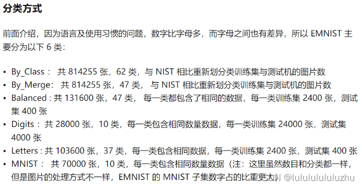
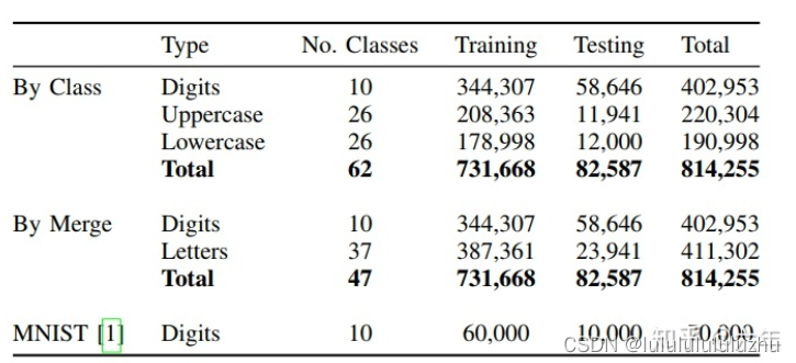
1. EMNIST
2. MNIST
手写数字数据集
类别:0~9 10个类别
训练集:60000张
测试集:10000张
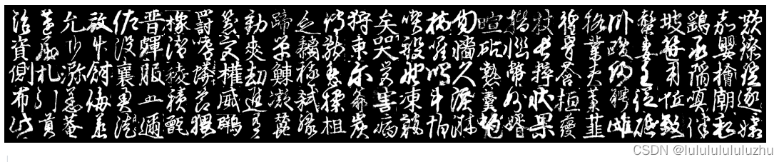
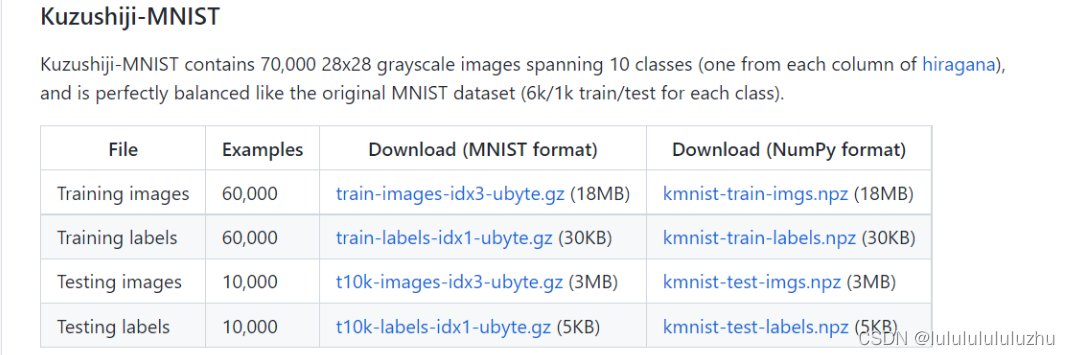
3. KMNIST
古日文数据集
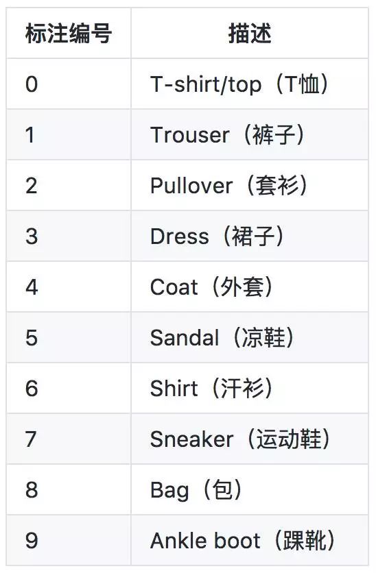
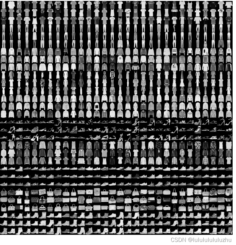
4. Fashion MNIST
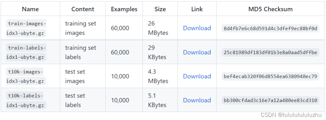
有10个类别:
手写数字数据集样式
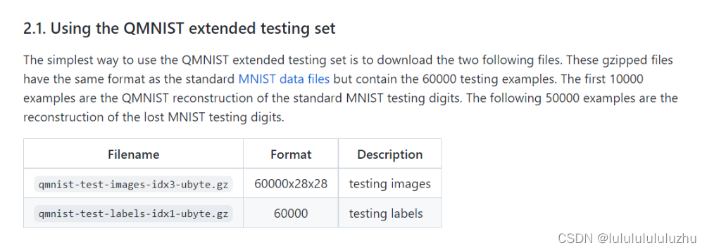
5. QMNIST
手写数字数据集
在测试集上对MNIST进行了补充,增加了50000张图片
训练集:60000张样本
测试集:60000张样本
6. SUHN
数据集内容来源于真实场景,是从谷歌街景图像中获得的门牌号。分成train,test,extra三个子集,各有73257,26032,531131个样本。样本包含0-9十个数字,1-9对应标签1-9,0对应标签10。
提供的数据有两种格式,第一种是压缩包,内含原始图片以及数字所在位置的检测框,需要更具体的信息查看上面的链接;如图
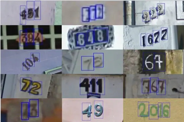
第二种是mat格式,每一个图片size为33232,仅含单个数字。一个样本对应4个维度,[:,:,:,i],对应的标签为y(i),如图
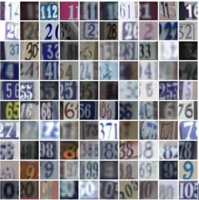
trochvision提供处理好的datasets类,图像为33232,像素值范围:0-255,0-9对应的标签是0-9。注意SVHN样本内含有干扰的数字信息。
7. USPS
USPS是美国邮政编码的信封手写数字。大小为[1,16,16]。提供的数据集有train/7291和test/2007。数据为归一化后的数据。0-9对应标签为0-9。
三、模型结构
1. alexnet:
可以训练1×28×28的灰度图片
class AlexNet(nn.Module): def __init__(self): super(AlexNet,self).__init__() # 由于MNIST为28x28, 而最初AlexNet的输入图片是227x227的。所以网络层数和参数需要调节 self.conv1 = nn.Conv2d(1, 32, kernel_size=3, padding=1) #AlexCONV1(3,96, k=11,s=4,p=0) self.pool1 = nn.MaxPool2d(kernel_size=2, stride=2)#AlexPool1(k=3, s=2) self.relu1 = nn.ReLU() # self.conv2 = nn.Conv2d(96, 256, kernel_size=5,stride=1,padding=2) self.conv2 = nn.Conv2d(32, 64, kernel_size=3, stride=1, padding=1)#AlexCONV2(96, 256,k=5,s=1,p=2) self.pool2 = nn.MaxPool2d(kernel_size=2,stride=2)#AlexPool2(k=3,s=2) self.relu2 = nn.ReLU() self.conv3 = nn.Conv2d(64, 128, kernel_size=3, stride=1, padding=1)#AlexCONV3(256,384,k=3,s=1,p=1) # self.conv4 = nn.Conv2d(384, 384, kernel_size=3, stride=1, padding=1) self.conv4 = nn.Conv2d(128, 256, kernel_size=3, stride=1, padding=1)#AlexCONV4(384, 384, k=3,s=1,p=1) self.conv5 = nn.Conv2d(256, 256, kernel_size=3, stride=1, padding=1)#AlexCONV5(384, 256, k=3, s=1,p=1) self.pool3 = nn.MaxPool2d(kernel_size=2, stride=2)#AlexPool3(k=3,s=2) self.relu3 = nn.ReLU() self.fc6 = nn.Linear(256*3*3, 1024) #AlexFC6(256*6*6, 4096) self.fc7 = nn.Linear(1024, 512) #AlexFC6(4096,4096) self.fc8 = nn.Linear(512, 10) #AlexFC6(4096,1000) def forward(self,x): x = self.conv1(x) x = self.pool1(x) x = self.relu1(x) x = self.conv2(x) x = self.pool2(x) x = self.relu2(x) x = self.conv3(x) x = self.conv4(x) x = self.conv5(x) x = self.pool3(x) x = self.relu3(x) x = x.view(-1, 256 * 3 * 3)#Alex: x = x.view(-1, 256*6*6) x = self.fc6(x) x = F.relu(x) x = self.fc7(x) x = F.relu(x) x = self.fc8(x) return x
网络结构:
index param.shape param.requires_grad 0 torch.Size([32, 1, 3, 3]) True 1 torch.Size([32]) True 2 torch.Size([64, 32, 3, 3]) True 3 torch.Size([64]) True 4 torch.Size([128, 64, 3, 3]) True 5 torch.Size([128]) True 6 torch.Size([256, 128, 3, 3]) True 7 torch.Size([256]) True 8 torch.Size([256, 256, 3, 3]) True 9 torch.Size([256]) True 10 torch.Size([1024, 2304]) True 11 torch.Size([1024]) True 12 torch.Size([512, 1024]) True 13 torch.Size([512]) True 14 torch.Size([10, 512]) True 15 torch.Size([10]) True —————— 8 层
在进行预训练时,冻结最后三个全连接层
2. Resnet:
类似Resnet的结构,可以训练1×28×28的灰度图片
class Basicblock(nn.Module): def __init__(self, in_planes, planes, stride=1): super(Basicblock, self).__init__() self.conv1 = nn.Sequential( nn.Conv2d(in_channels=in_planes, out_channels=planes, kernel_size=3, stride=stride, padding=1, bias=False), nn.BatchNorm2d(planes), nn.ReLU() ) self.conv2 = nn.Sequential( nn.Conv2d(in_channels=planes, out_channels=planes, kernel_size=3, stride=1, padding=1, bias=False), nn.BatchNorm2d(planes), ) if stride != 1 or in_planes != planes: self.shortcut = nn.Sequential( nn.Conv2d(in_channels=in_planes, out_channels=planes, kernel_size=3, stride=stride, padding=1), nn.BatchNorm2d(planes) ) else: self.shortcut = nn.Sequential() def forward(self, x): out = self.conv1(x) out = self.conv2(out) out += self.shortcut(x) out = F.relu(out) return out class ResNet(nn.Module): def __init__(self, block, num_block, num_classes): super(ResNet, self).__init__() self.in_planes = 16 self.conv1 = nn.Sequential( nn.Conv2d(in_channels=1, out_channels=16, kernel_size=3, stride=1, padding=1), nn.BatchNorm2d(16), nn.ReLU() ) self.maxpool = nn.MaxPool2d(kernel_size=3, stride=1, padding=1) self.block1 = self._make_layer(block, 16, num_block[0], stride=1) self.block2 = self._make_layer(block, 32, num_block[1], stride=2) self.block3 = self._make_layer(block, 64, num_block[2], stride=2) # self.block4 = self._make_layer(block, 512, num_block[3], stride=2) self.outlayer = nn.Linear(64, num_classes) def _make_layer(self, block, planes, num_block, stride): layers = [] for i in range(num_block): if i == 0: layers.append(block(self.in_planes, planes, stride)) else: layers.append(block(planes, planes, 1)) self.in_planes = planes return nn.Sequential(*layers) def forward(self, x): x = self.maxpool(self.conv1(x)) x = self.block1(x) # [200, 64, 28, 28] x = self.block2(x) # [200, 128, 14, 14] x = self.block3(x) # [200, 256, 7, 7] # out = self.block4(out) x = F.avg_pool2d(x, 7) # [200, 256, 1, 1] x = x.view(x.size(0), -1) # [200,256] out = self.outlayer(x) return out ResNet18 = ResNet(Basicblock, [1, 1, 1, 1], 10)
网络结构:
ResNet( (conv1): Sequential( (0): Conv2d(1, 16, kernel_size=(3, 3), stride=(1, 1), padding=(1, 1)) (1): BatchNorm2d(16, eps=1e-05, momentum=0.1, affine=True, track_running_stats=True) (2): ReLU() ) (maxpool): MaxPool2d(kernel_size=3, stride=1, padding=1, dilation=1, ceil_mode=False) (block1): Sequential( (0): Basicblock( (conv1): Sequential( (0): Conv2d(16, 16, kernel_size=(3, 3), stride=(1, 1), padding=(1, 1), bias=False) (1): BatchNorm2d(16, eps=1e-05, momentum=0.1, affine=True, track_running_stats=True) (2): ReLU() ) (conv2): Sequential( (0): Conv2d(16, 16, kernel_size=(3, 3), stride=(1, 1), padding=(1, 1), bias=False) (1): BatchNorm2d(16, eps=1e-05, momentum=0.1, affine=True, track_running_stats=True) ) (shortcut): Sequential() ) ) (block2): Sequential( (0): Basicblock( (conv1): Sequential( (0): Conv2d(16, 32, kernel_size=(3, 3), stride=(2, 2), padding=(1, 1), bias=False) (1): BatchNorm2d(32, eps=1e-05, momentum=0.1, affine=True, track_running_stats=True) (2): ReLU() ) (conv2): Sequential( (0): Conv2d(32, 32, kernel_size=(3, 3), stride=(1, 1), padding=(1, 1), bias=False) (1): BatchNorm2d(32, eps=1e-05, momentum=0.1, affine=True, track_running_stats=True) ) (shortcut): Sequential( (0): Conv2d(16, 32, kernel_size=(3, 3), stride=(2, 2), padding=(1, 1)) (1): BatchNorm2d(32, eps=1e-05, momentum=0.1, affine=True, track_running_stats=True) ) ) ) (block3): Sequential( (0): Basicblock( (conv1): Sequential( (0): Conv2d(32, 64, kernel_size=(3, 3), stride=(2, 2), padding=(1, 1), bias=False) (1): BatchNorm2d(64, eps=1e-05, momentum=0.1, affine=True, track_running_stats=True) (2): ReLU() ) (conv2): Sequential( (0): Conv2d(64, 64, kernel_size=(3, 3), stride=(1, 1), padding=(1, 1), bias=False) (1): BatchNorm2d(64, eps=1e-05, momentum=0.1, affine=True, track_running_stats=True) ) (shortcut): Sequential( (0): Conv2d(32, 64, kernel_size=(3, 3), stride=(2, 2), padding=(1, 1)) (1): BatchNorm2d(64, eps=1e-05, momentum=0.1, affine=True, track_running_stats=True) ) ) ) (outlayer): Linear(in_features=64, out_features=10, bias=True) ) ——————10 层
index  param.shape  param.requires_grad
0 torch.Size([16, 1, 3, 3]) True √
1 torch.Size([16]) True
2 torch.Size([16]) True
3 torch.Size([16]) True
4 torch.Size([16, 16, 3, 3]) True √
5 torch.Size([16]) True
6 torch.Size([16]) True
7 torch.Size([16, 16, 3, 3]) True √
8 torch.Size([16]) True
9 torch.Size([16]) True
10 torch.Size([32, 16, 3, 3]) True √
11 torch.Size([32]) True
12 torch.Size([32]) True
13 torch.Size([32, 32, 3, 3]) True √
14 torch.Size([32]) True
15 torch.Size([32]) True
16 torch.Size([32, 16, 3, 3]) True √
17 torch.Size([32]) True
18 torch.Size([32]) True
19 torch.Size([32]) True
20 torch.Size([64, 32, 3, 3]) True √
21 torch.Size([64]) True
22 torch.Size([64]) True
23 torch.Size([64, 64, 3, 3]) True √
24 torch.Size([64]) True
25 torch.Size([64]) True
26 torch.Size([64, 32, 3, 3]) True √
27 torch.Size([64]) True
28 torch.Size([64]) True
29 torch.Size([64]) True
30 torch.Size([10, 64]) True √
31 torch.Size([10]) True
在微调时,冻结最后两个卷积层和最后一层全连接层
3. MLPMixer:
MLP-Mixer主要包括三部分:Per-patch Fully-connected、Mixer Layer、分类器。

分类器:分类器部分采用传统的全局平均池化(GAP)+全连接层(FC)+Softmax的方式构成
Per-patch:具体来说,MLP-Mixer将输入图像相邻无重叠地划分为S个Patch,每个Patch通过MLP映射为一维特征向量,其中一维向量长度为C,最后将每个Patch得到的特征向量组合得到大小为S*C的 2D Table。
Mixer Layer:MLP-Mixer在Mixer Layer中使用分别使用token-mixing MLPs(图中MLP1)和channel-mixing MLPs(图中MLP2)对Table的列和行进行映射
观察Per-patch Fully-connected得到的Table会发现,Table的行代表了同一空间位置在不同通道上的信息,列代表了不同空间位置在同一通道上的信息。换句话说,对Table的每一行1*1 Conv 可以实现通道域的信息融合,对Table的每一列 实行 Self-Attention可以实现空间域的信息融合。
net = MLPMixer(
    image_size= 28,
    channels= 1,
    patch_size= 4,
    dim=128,
    depth= 1,
    num_classes= 10
)
Sequential(
  (0): Rearrange('b c (h p1) (w p2) -> b (h w) (p1 p2 c)', p1=4, p2=4)
  (1): Linear(in_features=16, out_features=128, bias=True)
  (2): Sequential(
    (0): PreNormResidual(
      (fn): Sequential(
        (0): Conv1d(49, 196, kernel_size=(1,), stride=(1,))
        (1): GELU()
        (2): Dropout(p=0.0, inplace=False)
        (3): Conv1d(196, 49, kernel_size=(1,), stride=(1,))
        (4): Dropout(p=0.0, inplace=False)
      )
      (norm): LayerNorm((128,), eps=1e-05, elementwise_affine=True)
    )
    (1): PreNormResidual(
      (fn): Sequential(
        (0): Linear(in_features=128, out_features=64, bias=True)
        (1): GELU()
        (2): Dropout(p=0.0, inplace=False)
        (3): Linear(in_features=64, out_features=128, bias=True)
        (4): Dropout(p=0.0, inplace=False)
      )
      (norm): LayerNorm((128,), eps=1e-05, elementwise_affine=True)
    )
  )
  (3): LayerNorm((128,), eps=1e-05, elementwise_affine=True)
  (4): Reduce('b n c -> b c', 'mean')
  (5): Linear(in_features=128, out_features=10, bias=True)
)
0 torch.Size([128, 16]) True
1 torch.Size([128]) True         ✔
2 torch.Size([196, 49, 1]) True
3 torch.Size([196]) True         ✔
4 torch.Size([49, 196, 1]) True
5 torch.Size([49]) True          ✔
6 torch.Size([128]) True
7 torch.Size([128]) True
8 torch.Size([64, 128]) True
9 torch.Size([64]) True          ✔
10 torch.Size([128, 64]) True
11 torch.Size([128]) True        ✔
12 torch.Size([128]) True
13 torch.Size([128]) True
14 torch.Size([128]) True
15 torch.Size([128]) True
16 torch.Size([10, 128]) True
17 torch.Size([10]) True          ✔
net = MLPMixer(
    image_size= 28,
    channels= 1,
    patch_size= 4,
    dim=128,
    depth= 2,
    num_classes= 10
)
Sequential(
  (0): Rearrange('b c (h p1) (w p2) -> b (h w) (p1 p2 c)', p1=4, p2=4)
  (1): Linear(in_features=16, out_features=128, bias=True)
  (2): Sequential(
    (0): PreNormResidual(
      (fn): Sequential(
        (0): Conv1d(49, 196, kernel_size=(1,), stride=(1,))
        (1): GELU()
        (2): Dropout(p=0.0, inplace=False)
        (3): Conv1d(196, 49, kernel_size=(1,), stride=(1,))
        (4): Dropout(p=0.0, inplace=False)
      )
      (norm): LayerNorm((128,), eps=1e-05, elementwise_affine=True)
    )
    (1): PreNormResidual(
      (fn): Sequential(
        (0): Linear(in_features=128, out_features=64, bias=True)
        (1): GELU()
        (2): Dropout(p=0.0, inplace=False)
        (3): Linear(in_features=64, out_features=128, bias=True)
        (4): Dropout(p=0.0, inplace=False)
      )
      (norm): LayerNorm((128,), eps=1e-05, elementwise_affine=True)
    )
  )
  (3): Sequential(
    (0): PreNormResidual(
      (fn): Sequential(
        (0): Conv1d(49, 196, kernel_size=(1,), stride=(1,))
        (1): GELU()
        (2): Dropout(p=0.0, inplace=False)
        (3): Conv1d(196, 49, kernel_size=(1,), stride=(1,))
        (4): Dropout(p=0.0, inplace=False)
      )
      (norm): LayerNorm((128,), eps=1e-05, elementwise_affine=True)
    )
    (1): PreNormResidual(
      (fn): Sequential(
        (0): Linear(in_features=128, out_features=64, bias=True)
        (1): GELU()
        (2): Dropout(p=0.0, inplace=False)
        (3): Linear(in_features=64, out_features=128, bias=True)
        (4): Dropout(p=0.0, inplace=False)
      )
      (norm): LayerNorm((128,), eps=1e-05, elementwise_affine=True)
    )
  )
  (4): LayerNorm((128,), eps=1e-05, elementwise_affine=True)
  (5): Reduce('b n c -> b c', 'mean')
  (6): Linear(in_features=128, out_features=10, bias=True)
)
0 torch.Size([128, 16]) True     ✔
1 torch.Size([128]) True
2 torch.Size([196, 49, 1]) True  ✔
3 torch.Size([196]) True
4 torch.Size([49, 196, 1]) True  ✔
5 torch.Size([49]) True
6 torch.Size([128]) True
7 torch.Size([128]) True
8 torch.Size([64, 128]) True     ✔
9 torch.Size([64]) True
10 torch.Size([128, 64]) True    ✔
11 torch.Size([128]) True
12 torch.Size([128]) True
13 torch.Size([128]) True
14 torch.Size([196, 49, 1]) True ✔
15 torch.Size([196]) True
16 torch.Size([49, 196, 1]) True ✔
17 torch.Size([49]) True
18 torch.Size([128]) True
19 torch.Size([128]) True
20 torch.Size([64, 128]) True    ✔
21 torch.Size([64]) True
22 torch.Size([128, 64]) True    ✔
23 torch.Size([128]) True
24 torch.Size([128]) True
25 torch.Size([128]) True
26 torch.Size([128]) True
27 torch.Size([128]) True
28 torch.Size([10, 128]) True    ✔
29 torch.Size([10]) True
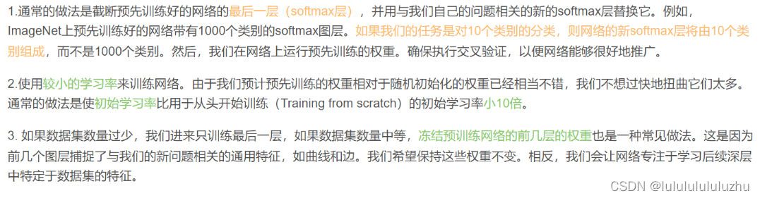
3. 微调的一些原则
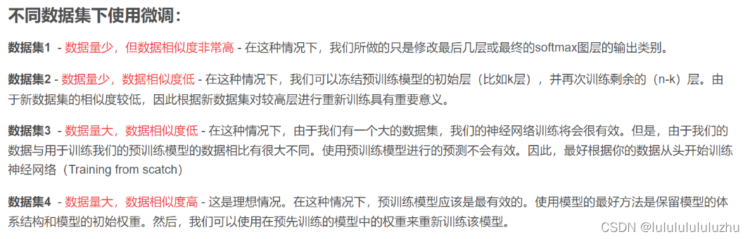
微调的一些注意事项:
四、预训练模型和微调模型:
1)预训练模型
-
pretrained model :KMNIST预训练alexnet
-
pretrained model: FMNIST 预训练 alexnet
-
pretrained model: KMNIST 预训练 Resnet
-
pretrained model: FMNIST 预训练 Resnet
......
| 精确度 | KMNIST预训练alexnet | FMNIST预训练alexnet | KMNIST预训练Resnet | FMNIST预训练Resnet | SVHN预训练Resnet | MNIST 预训练resnet | MNIST 预训练alexnet | USPS预训练resnet | USPS预训练alexnet |
|---|---|---|---|---|---|---|---|---|---|
| train accuracy | 98.65 | 92.67 | 99.19 | 95.77 | 0.9556 | 0.9951 | 0.9856 | 0.9995 | 0.9993 |
| test accuracy | 92.00 | 90.27 | 94.83 | 92.30 | 0.9368 | 0.9898 | 0.9821 | 0.9746 | 0.9721 |
2)微调模型
-
final model: KMNIST预训练alexnet , MNIST 微调
-
final model: FMNIST预训练alexnet , MNIST 微调
-
final model:FMNIST 预训练 Resnet , MNIST 微调
-
final model:KMNST 预训练 Resnet,MNIST微调
| fine with 60000MNIST | FMNIST预训练alexnet | KMNIST预训练alexnet | KMNIST预训练Resnet | FMNIST预训练Resnet |
|---|---|---|---|---|
| train accuracy | 95.99 | 98.77 | 98.20 | 94.59 |
| test accuracy | 92.33 | 97.45 | 97.98 | 94.40 |
使用少量的数据MNIST 集进行微调
补充实验:
-
10000张 MNIST 训练Resnet :
train acc = 0.9945 ; test acc = 0.9678
20000张 MNIST 训练Resnet :
train acc = 0.9959 ; test acc = 0.9804
-
10000张 MNIST 训练alexnet :
train acc = 0.9916; test acc = 0.9713
3. 20000张 MNIST 训练alexnet:
Traing Accuracy: 0.9883 ;Test Accuracy: 0.9779
| fine with MNIST | FMNIST预训练alexnet 20000MNIST-冻结8层 | KMNIST预训练alexnet 10000MNIST-冻结8层 | KMNIST预训练Resnet 10000MNIST-冻结23层 | FMNIST预训练Resnet 20000MNIST-冻结20层 |
|---|---|---|---|---|
| train accuracy | 0.9994 | 1.000 | 0.9965 | 0.9956 |
| test accuracy | 0.9342 | 0.9636 | 0.9734 | 0.9570 |
FMNIST预训练Resnet 10000MNIS微调-冻结23层 : train acc = 0.9862 ; test acc = 0.9342
FMNIST预训练Resnet 10000MNIS微调-冻结20层 : train acc = 0.9990 ; test acc = 0.9424
五、对抗攻击实验
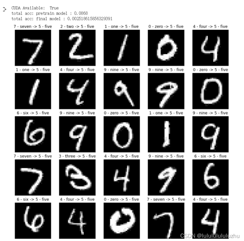
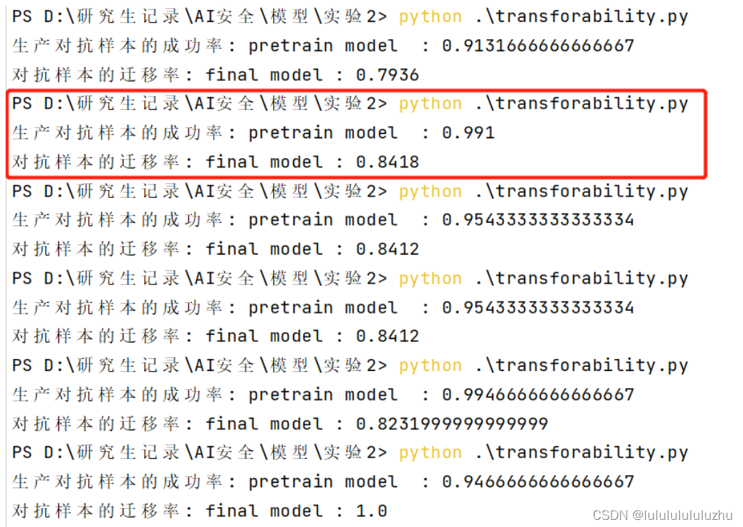
1. final_alexnet_KMNIST_MNIST
pre_alexnet_KMNIST and pre_alexnet_FMNIST and final_alexnet_KMNIST_MNIS
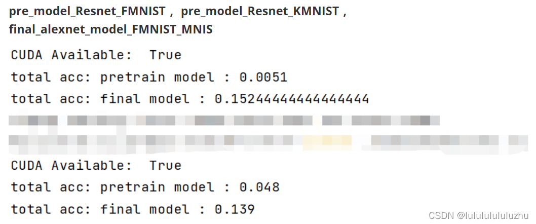
pre_model_Resnet_KMNIST ,pre_model_Resnet_FMNIST ,final_alexnet_model_KMNIST_MNIS
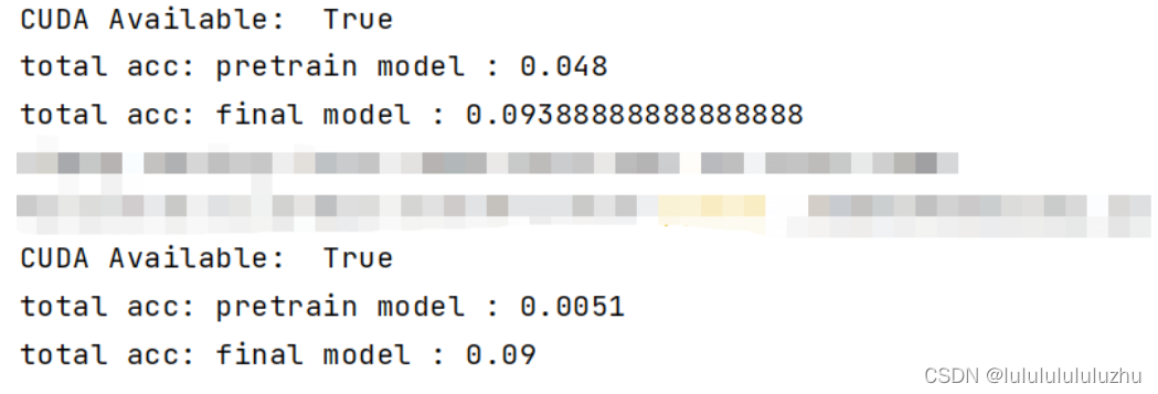
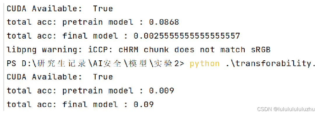
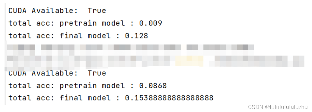
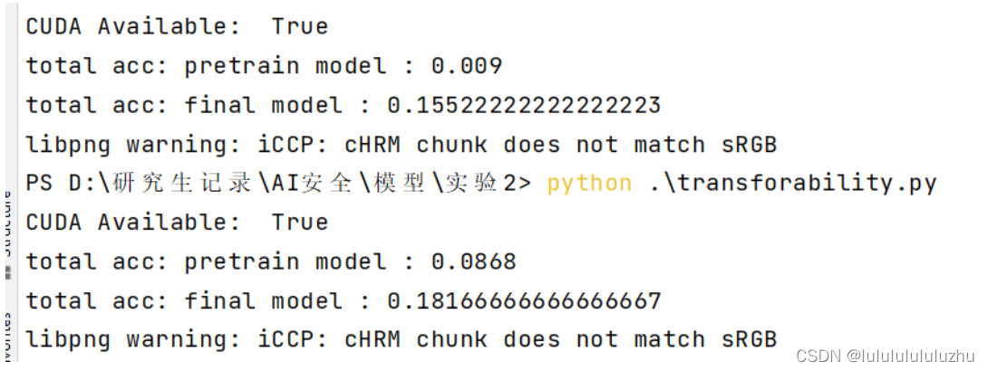
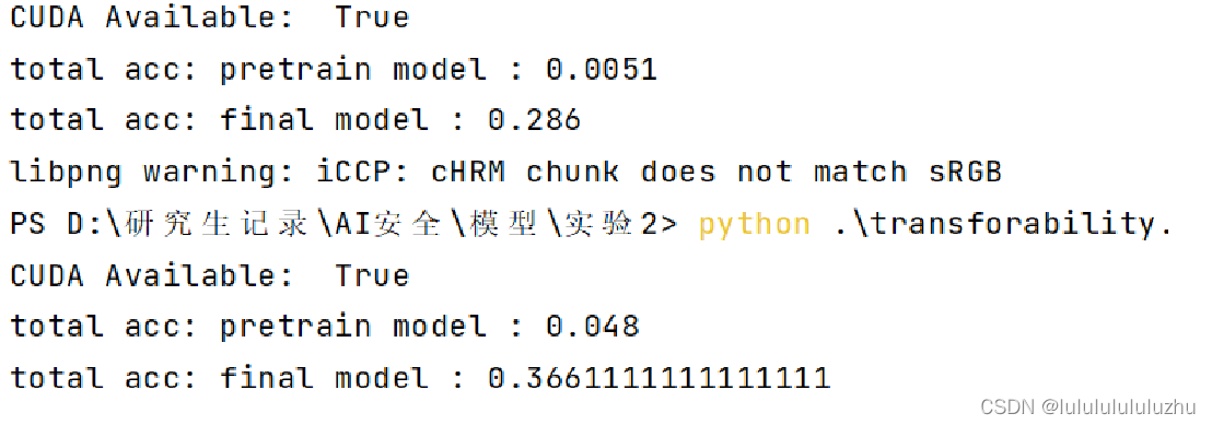
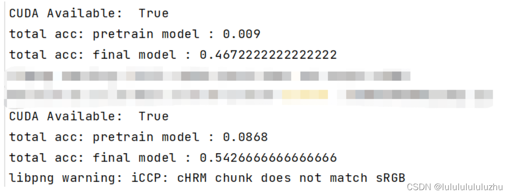
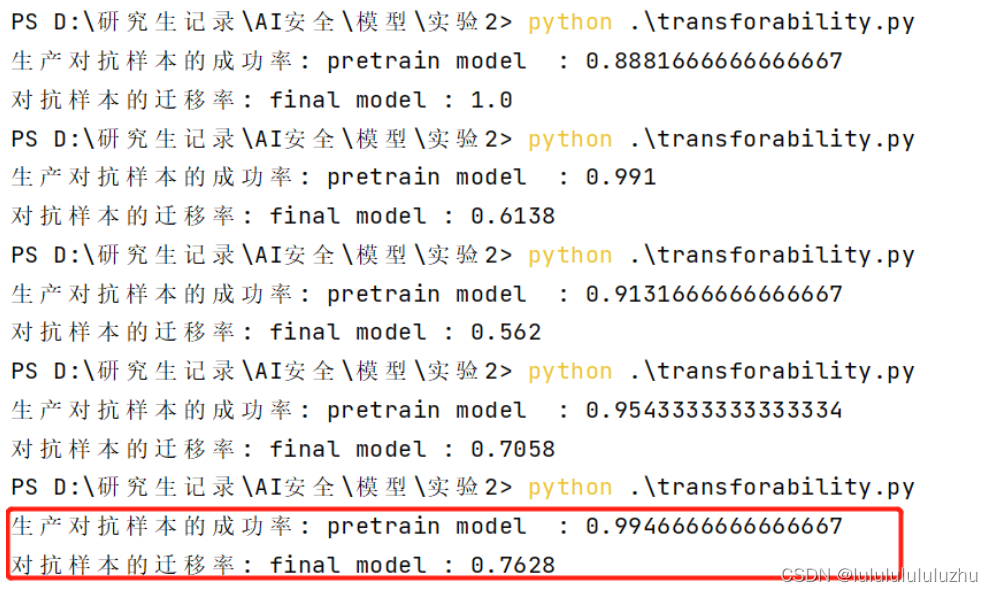
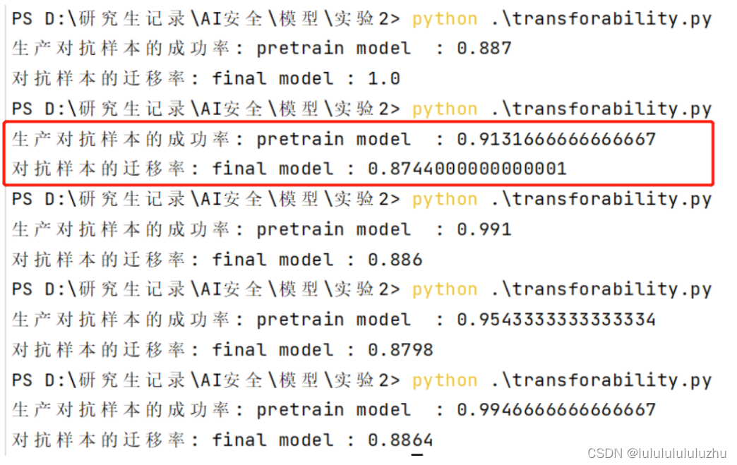
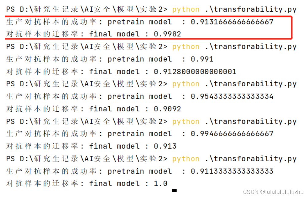
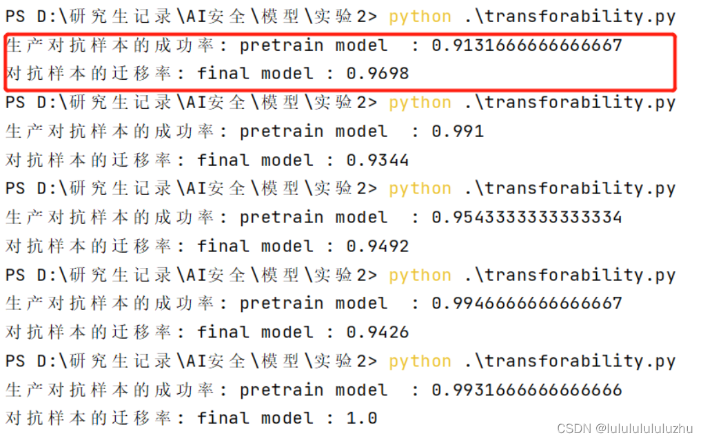
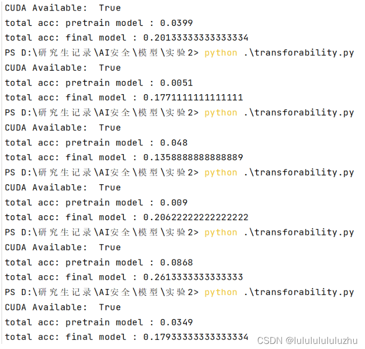
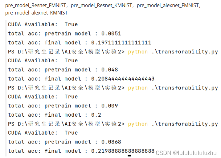
说明:total acc : pretrain model :代表预训练模型生成的对抗样本攻击自己得到的准确率
total acc : final model :代表预训练模型生成的对抗样本攻击微调模型得到的准确率
2. final_model_alexnet_FMNIST_MNIST
pre_model_alexnet_FMNIST and pre_model_alexnet_KMNIST and final_model_alexnet_FMNIST_MNIST
pre_model_Resnet_FMNIST ,pre_model_Resnet_KMNIST ,final_alexnet_model_FMNIST_MNIS
3. final_model_Resnet_KMNIST_MNIST
pre_model_Resnet_KMNIST ,pre_model_Resnet_FMNIST,final_model_Resnet_KMNIST_MNIST

pre_model_alexnet_FMNIST , pre_model_alexnet_KMNIST ,final_model_Resnet_KMNIST_MNIST
4. final_model_Resnet_FMNIST_MNIST
pre_model_Resnet_FMNIST ,pre_model_Resnet_KMNIST ,final_model_Resnet_FMNIST_MNIST
pre_model_alexnet_FMNIST , pre_model_alexnet_KMNIST ,final_model_Resnet_FMNIST_MNIST
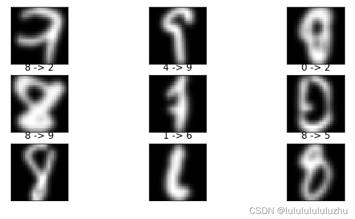
对抗样本示例:
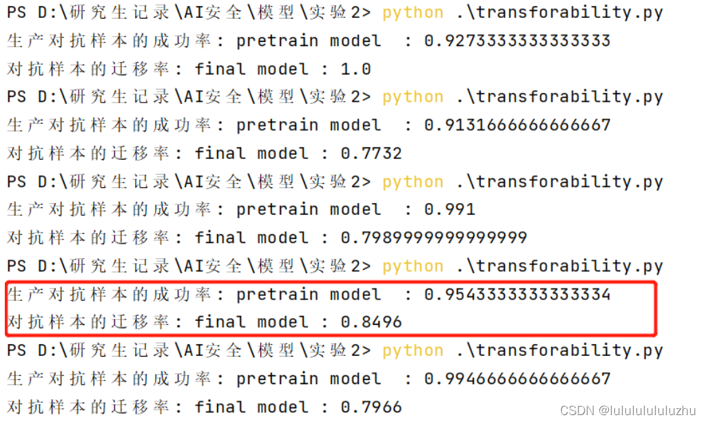
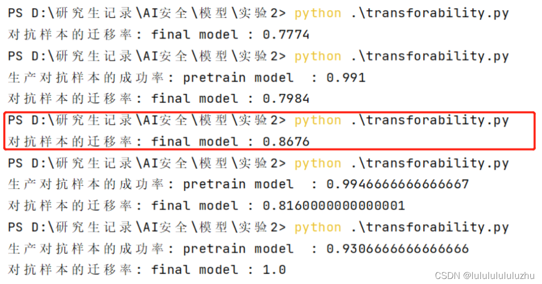
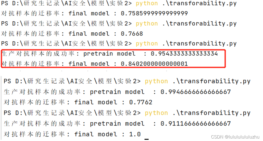
重做对抗攻击实验
以此按照目标模型,pre_model_alexnet_KMNIST,pre_model_alexnet_FMNIST,pre_model_Resnet_KMNIST,pre_model_Resnet_FMNIST 攻击目标模型,生产对抗样本5000张
1. final_model_Resnet_KMNIST_10000MNIST_train_0.9965_test_0.9734
final_model_Resnet_KMNIST_1000MNIST_train_0.9950_test_0.9420_23
final_model_Resnet_KMNIST_500MNIST_train_1.000_test_0.9160_23
2. final_model_Resnet_FMNIST_10000MNIST_train_0.9990_test_0.9424_20
3. final_model_alexnet_KMNIST_10000MNIST_train_1.000_test_0.9636_8
final_model_alexnet_KMNIST_10000MNIST_train_0.9997_test_0.9574_8
final_model_alexnet_KMNIST_10000MNIST_train_0.9999_test_0.9607_8
4. final_model_alexnet_FMNIST_20000MNIST_train_0.9994_test_0.9342

final_model_alexnet_FMNIST_20000MNIST_train_0.9520_0.8928_10
六、补充实验
1. EMNIST balanced pretrain model , MNIST(size=10000) fine tune model :
EMNIST : “balanced‘’
train data : 112800
test data :18800
classes : 47类 ['0', '1', '2', '3', '4', '5', '6', '7', '8', '9', 'A', 'B', 'C', 'D', 'E', 'F', 'G', 'H', 'I', 'J', 'K', 'L', 'M', 'N', 'O', 'P', 'Q', 'R', 'S', 'T', 'U', 'V', 'W', 'X', 'Y', 'Z', 'a', 'b', 'd', 'e', 'f', 'g', 'h', 'n', 'q', 'r', 't']
train accuray : 0.9843
test accuray : 0.9799
pre_model_Resnet_EMNIST_balance,pre_model_Resnet_FMNIST,pre_model_Resnet_KMNIST,pre_model_alexnet_FMNIST,pre_model_alexnet_KMNIST,pre_model_Resnet_EMNIST_letters
2. EMNIST letter pretrain model , MNIST(size=10000) fine tune model :
EMNIST : “balanced‘’
train data : 124800
test data : 20800
classes : 27类 ['N/A', 'a', 'b', 'c', 'd', 'e', 'f', 'g', 'h', 'i', 'j', 'k', 'l', 'm', 'n', 'o', 'p', 'q', 'r', 's', 't', 'u', 'v', 'w', 'x', 'y', 'z']
train accuray : 0.9821
test accuray : 0.9765
pre_model_Resnet_FMNIST,pre_model_Resnet_KMNIST,pre_model_alexnet_FMNIST,pre_model_alexnet_KMNIST
·


 被折叠的 条评论
为什么被折叠?
被折叠的 条评论
为什么被折叠?
 到【灌水乐园】发言


