Numpy学习笔记3--常用函数2_np.cov aweight-CSDN博客

本文链接：https://blog.csdn.net/luoyu_bie/article/details/79783882

真实波动幅度均值-主要演示maximum函数

# In[1]:
import numpy as np

# In[2]:
h,l,c = np.loadtxt('data/data.csv',delimiter=',',usecols=(4,5,6),unpack=True)

# In[3]:
#ATR 基于N个交易日的最高价和最低价进行计算，通常取近20个交易日
N = 20
h = h[-N:]
l = l[-N:]

# In[4]:
#前一个交易日的收盘价
previousclose = c[-N-1:-1]

# In[5]:
#h-l 当日股价范围
#h-previousclose 当日最高价与前一日收盘价之差
#previousclose - l 前一日收盘价与当日最低价之差

# In[6]:
truerange = np.maximum(h-l,h-previousclose,previousclose-l)


# In[7]:
print truerange
# Out[7]:
[  4.26   2.77   2.42   5.     3.75   9.98   7.68   6.03   6.78   5.55
   6.89   8.04   5.95   7.67   2.54  10.36   5.15   4.16   4.87   7.32]

# In[8]:
atr = np.zeros(N)

# In[9]:
atr[0] = np.mean(truerange)

# In[10]:
for i in range(1,N):
    atr[i] = (N-1)*atr[i-1] + truerange[i]
    atr[i] /= N

# In[11]:
atr
# Out[11]:
array([ 5.8585    ,  5.704075  ,  5.53987125,  5.51287769,  5.4247338 ,
        5.65249711,  5.75387226,  5.76767864,  5.81829471,  5.80487998,
        5.85913598,  5.96817918,  5.96727022,  6.05240671,  5.87678637,
        6.10094705,  6.0533997 ,  5.95872972,  5.90429323,  5.97507857])

简单的移动平均线

# In[12]:
N = 5
weights = np.ones(N)/N
print weights

# In[13]:
c = np.loadtxt('data/data.csv',delimiter=',',usecols=(6,),unpack=True)

# In[14]:
sma = np.convolve(weights,c)[N-1:-N+1]

# In[15]:
import matplotlib.pyplot as plt
t = np.arange(N-1,len(c))
plt.plot(t,c[N-1:],color='g',linewidth=1.0)
plt.plot(t,sma,color='r',linewidth=2.0)
plt.show()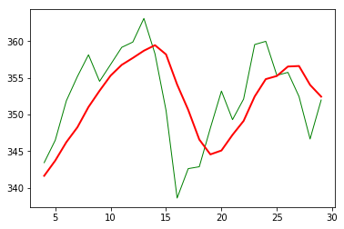

指数移动平均线

# In[16]:
x = np.arange(5)
print "Exp ",np.exp(x)
# Out[16]:
Exp  [  1.           2.71828183   7.3890561   20.08553692  54.59815003]

# In[17]:
print "Linspace ",np.linspace(-1,0,5)
# Out[17]:
Linspace  [-1.   -0.75 -0.5  -0.25  0.  ]

# In[18]:
N = 5
weights = np.exp(np.linspace(-1,0,N))
weights /= weights.sum()
print "Weights ",weights
# Out[18]:
Weights  [ 0.11405072  0.14644403  0.18803785  0.24144538  0.31002201]

# In[19]:
c = np.loadtxt('data/data.csv',delimiter=',',usecols=(6,),unpack=True)
ema = np.convolve(weights,c)[N-1:-N+1]
t = np.arange(N-1,len(c))
plt.plot(t,c[N-1:],color='g',linewidth=1.0)
plt.plot(t,ema,color='r',linewidth=2.0)
plt.show()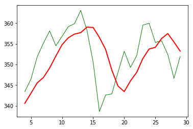

绘制布林带

# In[20]:
deviation = []
C = len(c)
for i in range(N-1,C):
    if i + N <C:
        dev = c[i:i+N]
    else:
        dev = c[-N:]
    averages = np.zeros(N)
    averages.fill(sma[i - N - 1])
    dev = dev - averages 
    dev = dev ** 2
    dev = np.sqrt(np.mean(dev))
    deviation.append(dev)
deviation = 2 * np.array(deviation)
print len(deviation),len(sma)
upperBB = sma + deviation
lowerBB = sma - deviation

c_slice = c[N-1:]
between_bands = np.where((c_slice < upperBB) & (c_slice > lowerBB))

print lowerBB[between_bands]
print c[between_bands]
print upperBB[between_bands]
between_bands = len(np.ravel(between_bands))
print "Ratio between bands", float(between_bands)/len(c_slice)

t = np.arange(N - 1, C)
plt.plot(t, c_slice, lw=1.0)
plt.plot(t, sma, lw=2.0)
plt.plot(t, upperBB, lw=3.0)
plt.plot(t, lowerBB, lw=4.0)
plt.show()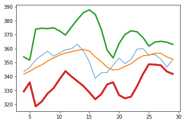

用线性模型预测价格

# In[21]:
b = c[-N:]
b = b[::-1]
print "b ",b
# Out[21]:
b  [ 351.99  346.67  352.47  355.76  355.36]

# In[22]:
A = np.zeros((N,N),float)
print A
# Out[22]:
[[ 0.  0.  0.  0.  0.]
 [ 0.  0.  0.  0.  0.]
 [ 0.  0.  0.  0.  0.]
 [ 0.  0.  0.  0.  0.]
 [ 0.  0.  0.  0.  0.]]

# In[23]:
#用b向量中的N个股价值填充数组A
for i in range(N):
    A[i,] = c[-N-1-i:-1-i]
print A
# Out[23]:
[[ 360.    355.36  355.76  352.47  346.67]
 [ 359.56  360.    355.36  355.76  352.47]
 [ 352.12  359.56  360.    355.36  355.76]
 [ 349.31  352.12  359.56  360.    355.36]
 [ 353.21  349.31  352.12  359.56  360.  ]]

# In[24]:
#求线性回归函数的系数，残差平方和数组，矩阵A的秩，A的奇异值
(x,residuals,rank,s) = np.linalg.lstsq(A,b)
print x,residuals,rank,s
# Out[24]:
[ 0.78111069 -1.44411737  1.63563225 -0.89905126  0.92009049] [] 5 [  1.77736601e+03   1.49622969e+01   8.75528492e+00   5.15099261e+00
   1.75199608e+00]

# In[25]:
#numpy.dot()计算向量的点积，即对下一个收盘价进行预测
print np.dot(b,x)
# Out[25]:
357.939161015

绘制趋势线

# In[26]:
#趋势线，是根据股价走势图上很多所谓的枢轴点绘成的曲线，
#描绘的是价格变化的趋势

# In[27]:
#假设枢轴点等于最高价、最低价、收盘价的算数平均值
h,l,c = np.loadtxt('data/data.csv',delimiter=',',usecols=(4,5,6),unpack=True)
pivots = (h+l+c)/3
print pivots
# Out[27]:
[ 338.01        337.88666667  343.88666667  344.37333333  342.07666667
  345.57        350.92333333  354.29        357.34333333  354.18
  356.06333333  358.45666667  359.14        362.84333333  358.36333333
  353.19333333  340.57666667  341.95666667  342.13333333  347.13
  353.12666667  350.90333333  351.62333333  358.42333333  359.34666667
  356.11333333  355.13666667  352.61        347.11333333  349.77      ]

# In[28]:
#支撑位是指在股价下跌时可能遇到支撑，从而止跌回稳前的最低价位. 
#阻力位则是指在股价上升时可能遇到压力，从而反转下跌前的最高价位

# In[29]:
#定义一个函数用直线y=ax + b 来拟合数据
def fit_line(t,y):
    A = np.vstack([t,np.ones_like(t)]).T
    return np.linalg.lstsq(A,y)[0]

# In[30]:
#假设支撑位在枢轴点下方一个当日股价区间的位置
#阻力位在枢轴点上方一个当日股价区间的位置
#据此拟合支撑位与阻力位的趋势线
t = np.arange(len(c))
sa,sb = fit_line(t,pivots-(h-l))
ra,rb = fit_line(t,pivots+(h-l))
support = sa*t +sb
resistance = ra*t + rb

# In[31]:
#判断数据点是否位于两条趋势线之间
condition = (c>support) & (c<resistance)
print "Condition ",condition
between_bands = np.where(condition)
# Out[31]:
Condition  [False False  True  True  True  True  True False False  True False False
 False False False  True False False False  True  True  True  True False
 False  True  True  True False  True]

# In[32]:
#复查具体取值
print support[between_bands]
print c[between_bands]
print resistance[between_bands]
# Out[32]:
[ 341.92421382  342.19081893  342.45742405  342.72402917  342.99063429
  343.79044964  345.39008034  346.4565008   346.72310592  346.98971104
  347.25631615  348.0561315   348.32273662  348.58934174  349.12255197]
[ 345.03  344.32  343.44  346.5   351.88  354.54  350.56  348.16  353.21
  349.31  352.12  355.36  355.76  352.47  351.99]
[ 352.61688271  352.90732765  353.19777259  353.48821753  353.77866246
  354.64999728  356.39266691  357.55444667  357.84489161  358.13533655
  358.42578149  359.2971163   359.58756124  359.87800618  360.45889606]

# In[33]:
#where函数返回的是秩为2的数组，需要用ravel展平
between_bands = len(np.ravel(between_bands))
print "Number points between bands ",between_bands
print "Ratio betwwen bands ",float(between_bands)/len(c)
# Out[33]:
Number points between bands  15
Ratio betwwen bands  0.5

# In[34]:
#此时得到一个新的预测模型，可用于预测下一个交易日的阻力位与支撑位
print "Tomorrows support ",sa*(t[-1]+1)+sb
print "Tomorrows resistance ",ra*(t[-1]+1) + rb
# Out[34]:
Tomorrows support  349.389157088
Tomorrows resistance  360.749340996

# In[35]:
#计算支撑位与阻力位之间数据点个数
#intersect1d 函数返回一个由两个数组的所有共同元素构成的数组
a1 = c[c>support]
a2 = c[c<resistance]
print "支撑位与阻力位之间数据点个数：",len(np.intersect1d(a1,a2))
# Out[35]:
支撑位与阻力位之间数据点个数： 15

# In[36]:
#绘制结果图
import matplotlib.pyplot as plt
plt.plot(t,c)
plt.plot(t,support)
plt.plot(t,resistance)
plt.show()

数组的修剪和压缩

# In[37]:
#clip方法返回一个修剪过的数组，即把所有比给定最大值还大的元素设定为给定的最大值
#而所有比给定最小值还小的元素设为给定的最小值
a = np.arange(8)
print "a= ",a
print "Clipped ",a.clip(2,6)
# Out[37]:
a=  [0 1 2 3 4 5 6 7]
Clipped  [2 2 2 3 4 5 6 6]

# In[38]:
#compress 方法返回一个根据给定条件筛选后的数组
a = np.arange(8)
print "a=",a
print "Compressed",a.compress(a>4)
# Out[38]:
a= [0 1 2 3 4 5 6 7]
Compressed [5 6 7]

# ### 计算阶乘

# In[39]:
#prod 可以计算数组中所有数据的乘积，以此来计算阶乘
b = np.arange(1,9)
print "b = ",b
print "8的阶乘：",b.prod()
# Out[39]:
b =  [1 2 3 4 5 6 7 8]
8的阶乘： 40320

# In[40]:
#cumprod 可以计算数组的累积乘积
print "累积乘积：",b.cumprod()
# Out[40]:
累积乘积： [    1     2     6    24   120   720  5040 40320]