从0-1实现大模型-CSDN博客

本文链接：https://blog.csdn.net/m0_37156901/article/details/139436492

输入数据准备

滑动窗口造数据 Data sampling with a sliding window

数据加载器的输出DataLoader

位置编码Encoding word positions

github: LLMs-from-scratch/ch02/01_main-chapter-code

LLM Visualization

输入数据准备

滑动窗口造数据 Data sampling with a sliding window

We train LLMs to generate one word at a time, so we want to prepare the training data accordingly where the next word in a sequence represents the target to predict:

 and ---->  established
 and established ---->  himself
 and established himself ---->  in
 and established himself in ---->  a

数据加载器的输出DataLoader

批量Batch的输出形式是：

Inputs:
 tensor([[992, 993, 994, 995],
        [996, 997, 998, 999]])

Targets:
 tensor([[ 993,  994,  995,  996],
        [ 997,  998,  999, 1000]])
无需Batch输出的单条形式：
[tensor([[0, 1, 2, 3]]), tensor([[1, 2, 3, 4]])]
[tensor([[1, 2, 3, 4]]), tensor([[2, 3, 4, 5]])]

位置编码Encoding word positions

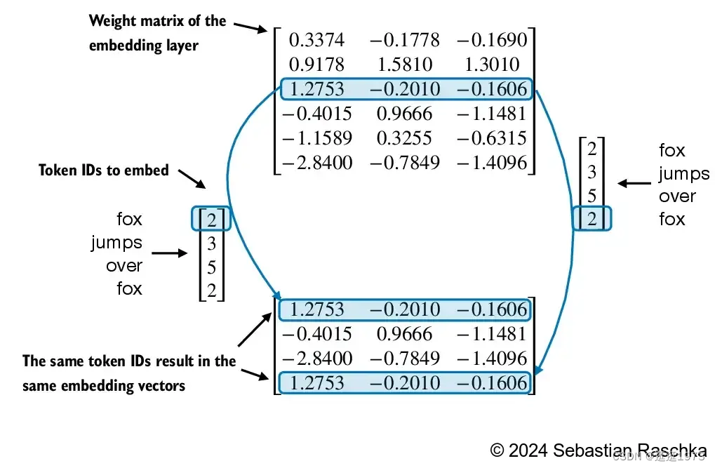
嵌入层将标识符转换为相同的向量表示，无论它们在输入序列中的位置如何：

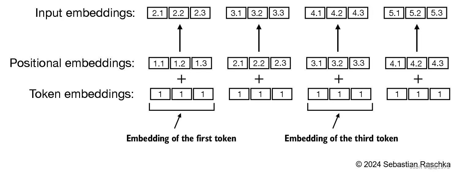
位置嵌入与标记嵌入向量相结合，形成大型语言模型的输入嵌入。

自注意力机制

点积的原理

Q*K 这个点积操作，这是一种通用且简单的方法，确保每个输出元素都能受到输入向量中所有元素的影响（其中的影响由权重决定）。因此，它在神经网络中经常出现。

点积是衡量两个向量之间相似性的一种方式。如果它们非常相似，点积会很大。如果它们非常不同，点积会很小或为负。

我们对Q、K、V向量的每个输出单元重复此操作：

QKV的原理

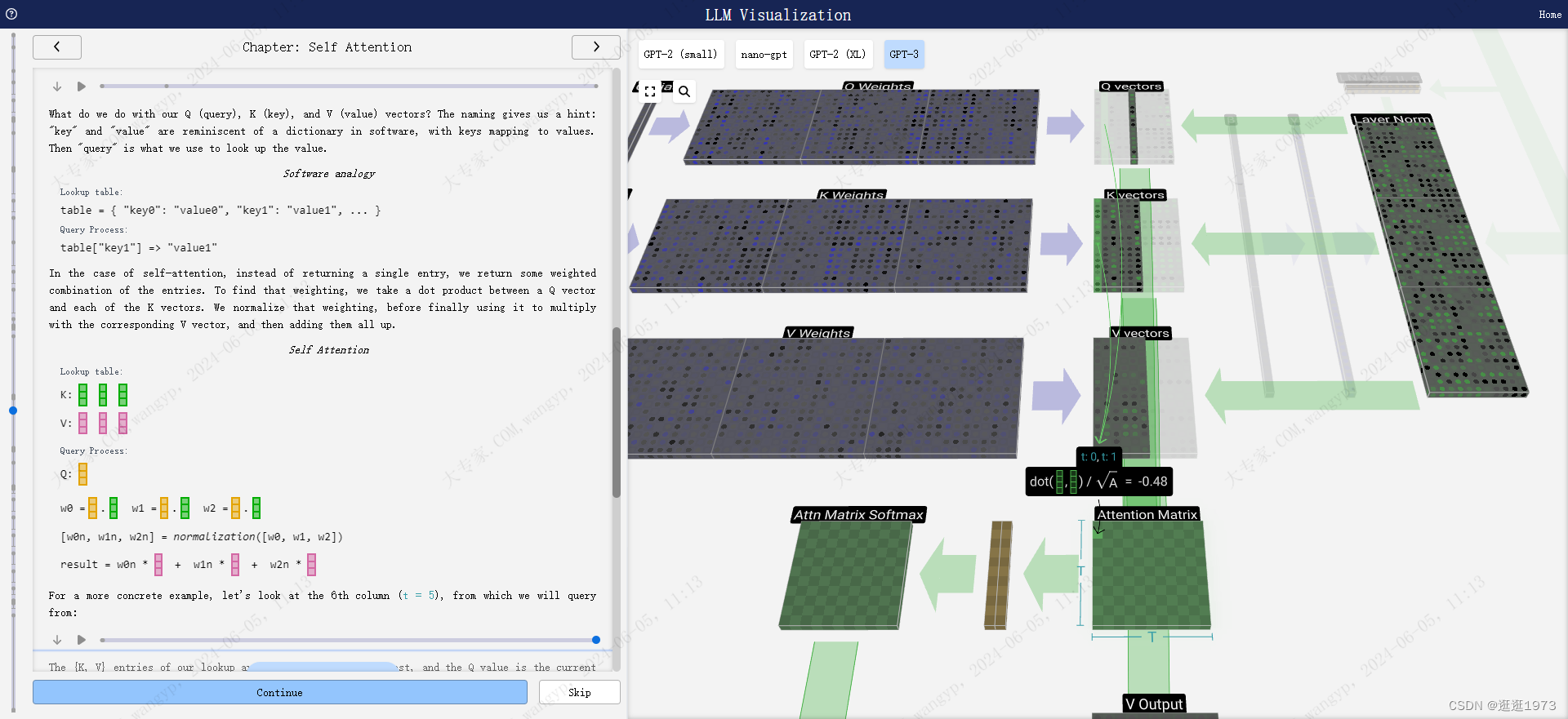
我们的Q（查询）、K（键）和V（值）向量是用来做什么的？命名给我们提供了一个提示：“键”和“值”让人想起软件中的字典，键映射到值。然后“查询”是我们用来查找值的工具。

软件类比：查找表： table = { "key0": "value0", "key1": "value1", ... } 查询过程： table["key1"] => "value1"

在自注意力的情况下，我们不是返回单个条目，而是返回条目的某种加权组合。为了找到那个加权，我们取Q向量和每个K向量之间的点积。我们规范化那个加权，然后最后用它来乘以相应的V向量，并将它们全部加起来。

我们的查找表中的{K, V}条目是过去的6列，而Q值是当前时间。

我们首先计算当前列（t = 5）的Q向量与之前每列的K向量之间的点积。然后将这些点积存储在注意力矩阵中相应的行（t = 5）。

实现代码

class CausalAttention(nn.Module):

    def __init__(self, d_in, d_out, context_length,
                 dropout, qkv_bias=False):
        super().__init__()
        self.d_out = d_out
        self.W_query = nn.Linear(d_in, d_out, bias=qkv_bias)
        self.W_key   = nn.Linear(d_in, d_out, bias=qkv_bias)
        self.W_value = nn.Linear(d_in, d_out, bias=qkv_bias)
        self.dropout = nn.Dropout(dropout) # New
        self.register_buffer('mask', torch.triu(torch.ones(context_length, context_length), diagonal=1)) # New

    def forward(self, x):
        b, num_tokens, d_in = x.shape # New batch dimension b
        keys = self.W_key(x)
        queries = self.W_query(x)
        values = self.W_value(x)

        attn_scores = queries @ keys.transpose(1, 2) # Changed transpose
        attn_scores.masked_fill_(  # New, _ ops are in-place
            self.mask.bool()[:num_tokens, :num_tokens], -torch.inf) 
        attn_weights = torch.softmax(
            attn_scores / keys.shape[-1]**0.5, dim=-1
        )
        attn_weights = self.dropout(attn_weights) # New

        context_vec = attn_weights @ values
        return context_vec

torch.manual_seed(123)

context_length = batch.shape[1]
ca = CausalAttention(d_in, d_out, context_length, 0.0)

context_vecs = ca(batch)

print(context_vecs)
print("context_vecs.shape:", context_vecs.shape)

Multi-head Attention

这就是自注意力层中一个头的处理过程。因此，自注意力的主要目标是每一列都想要从其他列中找到相关信息并提取它们的值，这是通过将其查询向量与那些其他列的键向量进行比较来实现的。加上的一个限制是，它只能查看过去。

多头注意力机制的主要思想是使用不同的、学习得到的线性投影并行地多次运行注意力机制。这使得模型能够同时从不同的位置关注来自不同表示子空间的信息。

class MultiHeadAttentionWrapper(nn.Module):

    def __init__(self, d_in, d_out, context_length, dropout, num_heads, qkv_bias=False):
        super().__init__()
        self.heads = nn.ModuleList(
            [CausalAttention(d_in, d_out, context_length, dropout, qkv_bias) 
             for _ in range(num_heads)]
        )

    def forward(self, x):
        return torch.cat([head(x) for head in self.heads], dim=-1)


torch.manual_seed(123)

context_length = batch.shape[1] # This is the number of tokens
d_in, d_out = 3, 2
mha = MultiHeadAttentionWrapper(
    d_in, d_out, context_length, 0.0, num_heads=2
)

context_vecs = mha(batch)

print(context_vecs)
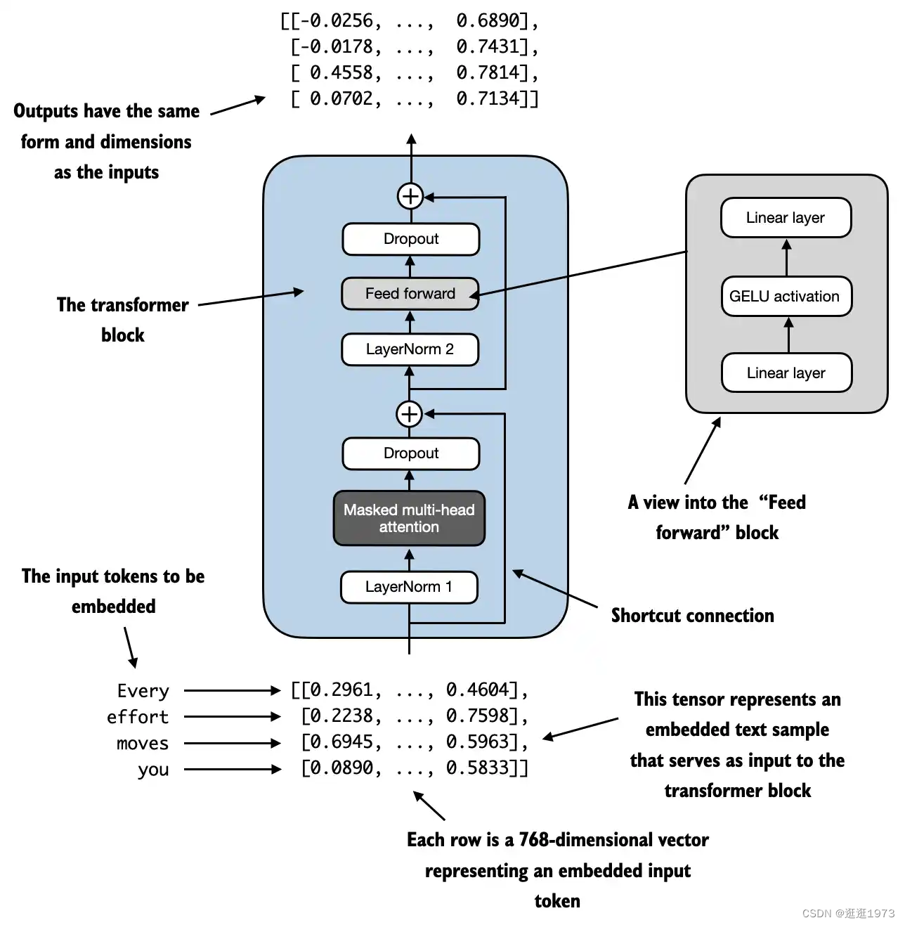
print("context_vecs.shape:", context_vecs.shape)

这就是一个完整的Transformer块！

这些块构成了任何GPT模型的主体，并会重复多次，一个块的输出会作为下一个块的输入，继续沿着残差路径前进。

正如在深度学习中常见的那样，很难确切地说这些层在做什么，但我们有一些大致的想法：早期层倾向于专注于学习低级特征和模式，而后期层则学习识别和理解更高层次的抽象和关系。在自然语言处理的背景下，较低层可能学习语法、句法和简单的词汇关联，而较高层可能捕捉更复杂的语义关系、话语结构和依赖上下文的含义。

线性层

最后，我们来到了模型的末端。最终的Transformer块的输出会通过一个层归一化，然后我们使用一个线性变换（矩阵乘法），这次没有偏置项。

这次最终的变换将每个列向量从长度C变换到长度nvocab。因此，它实际上是为每个列的词汇表中的每个词生成一个分数。这些分数有一个特殊的名字：logits。

"Logits"这个名字来源于"log-odds"，即每个标记的赔率的对数。"Log"被使用是因为我们接下来应用的softmax会进行指数化以转换为"赔率"或概率。

为了将这些分数转换为漂亮的概率，我们通过一个softmax操作传递它们。现在，对于每个列，我们都有一个模型分配给词汇表中每个词的概率。

在这个特定的模型中，它有效地学习了所有如何排序三个字母的问题的答案，所以概率严重偏向于正确答案。

当我们按时间顺序运行模型时，我们使用最后一列的概率来确定要添加到序列中的下一个标记。例如，如果我们向模型提供了六个标记，我们将使用第六列的输出概率。

这个列的输出是一系列概率，我们实际上必须选择其中之一作为序列中的下一个。我们通过"从分布中采样"来做到这一点。也就是说，我们根据其概率加权随机选择一个标记。例如，一个有0.9概率的标记将有90%的机会被选择。

然而，这里还有其他选项，比如总是选择概率最高的标记。

我们还可以通过使用温度参数来控制分布的"平滑度"。较高的温度会使分布更加均匀，而较低的温度会使它更集中在最高概率的标记上。

我们通过在应用softmax之前将logits（线性变换的输出）除以温度来做到这一点。由于softmax中的指数化对较大的数字有很大的影响，使它们更接近会减少这种效果。

Finally, we come to the end of the model. The output of the final transformer block is passed through a layer normalization, and then we use a linear transformation (matrix multiplication), this time without a bias.

This final transformation takes each of our column vectors from length C to length nvocab. Hence, it's effectively producing a score for each word in the vocabulary for each of our columns. These scores have a special name: logits.

The name "logits" comes from "log-odds," i.e., the logarithm of the odds of each token. "Log" is used because the softmax we apply next does an exponentiation to convert to "odds" or probabilities.

To convert these scores into nice probabilities, we pass them through a softmax operation. Now, for each column, we have a probability the model assigns to each word in the vocabulary.

In this particular model, it has effectively learned all the answers to the question of how to sort three letters, so the probabilities are heavily weighted toward the correct answer.

When we're stepping the model through time, we use the last column's probabilities to determine the next token to add to the sequence. For example, if we've supplied six tokens into the model, we'll use the output probabilities of the 6th column.

This column's output is a series of probabilities, and we actually have to pick one of them to use as the next in the sequence. We do this by "sampling from the distribution." That is, we randomly choose a token, weighted by its probability. For example, a token with a probability of 0.9 will be chosen 90% of the time.

There are other options here, however, such as always choosing the token with the highest probability.

We can also control the "smoothness" of the distribution by using a temperature parameter. A higher temperature will make the distribution more uniform, and a lower temperature will make it more concentrated on the highest probability tokens.

We do this by dividing the logits (the output of the linear transformation) by the temperature before applying the softmax. Since the exponentiation in the softmax has a large effect on larger numbers, making them all closer together will reduce this effect.