Python创建知识图，分析并训练嵌入模型（不连接数据库）

引用自  知识图谱入门：使用Python创建知识图，分析并训练嵌入模型_python 图嵌入实战-CSDN博客

目录

1.加载数据

2.创建一个NetworkX图(G)来表示KG。

3.绘制节点(实体)和边(关系)以及它们的标签。

 4.进行图谱分析

（1）查看节点和边

（2）节点中心性分析（Degree centrality、Betweenness centrality、Closeness centrality ）

（3）将上述节点中心性分析进行可视化

（4）最短路径分析

5.图嵌入（暂时用不到，不学习，有需要的可以去看原链接）

---

1.加载数据

 import pandas as pd
 
 # Define the heads, relations, and tails
 head = ['drugA', 'drugB', 'drugC', 'drugD', 'drugA', 'drugC', 'drugD', 'drugE', 'gene1', 'gene2','gene3', 'gene4', 'gene50', 'gene2', 'gene3', 'gene4']
 relation = ['treats', 'treats', 'treats', 'treats', 'inhibits', 'inhibits', 'inhibits', 'inhibits', 'associated', 'associated', 'associated', 'associated', 'associated', 'interacts', 'interacts', 'interacts']
 tail = ['fever', 'hepatitis', 'bleeding', 'pain', 'gene1', 'gene2', 'gene4', 'gene20', 'obesity', 'heart_attack', 'hepatitis', 'bleeding', 'cancer', 'gene1', 'gene20', 'gene50']
 
 # Create a dataframe
 df = pd.DataFrame({'head': head, 'relation': relation, 'tail': tail})
 df

2.创建一个NetworkX图(G)来表示KG。

DataFrame (df)中的每一行都对应于KG中的三元组(头、关系、尾)。add_edge函数在头部和尾部实体之间添加边，关系作为标签。

 import networkx as nx
 import matplotlib.pyplot as plt
 
 # Create a knowledge graph
 G = nx.Graph()
 for _, row in df.iterrows():
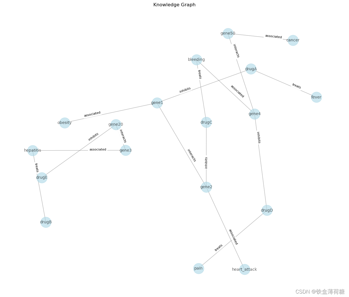
     G.add_edge(row['head'], row['tail'], label=row['relation'])

3.绘制节点(实体)和边(关系)以及它们的标签。

 # Visualize the knowledge graph
 pos = nx.spring_layout(G, seed=42, k=0.9)
 labels = nx.get_edge_attributes(G, 'label')
 plt.figure(figsize=(12, 10))
 nx.draw(G, pos, with_labels=True, font_size=10, node_size=700, node_color='lightblue', edge_color='gray', alpha=0.6)
 nx.draw_networkx_edge_labels(G, pos, edge_labels=labels, font_size=8, label_pos=0.3, verticalalignment='baseline')
 plt.title('Knowledge Graph')
 plt.show()

 4.进行图谱分析

（1）查看节点和边

对于知识图谱KG，可以做的第一件事是查看它有多少个节点和边，并分析它们之间的关系。

 num_nodes = G.number_of_nodes()
 num_edges = G.number_of_edges()
 print(f'Number of nodes: {num_nodes}')
 print(f'Number of edges: {num_edges}')
 print(f'Ratio edges to nodes: {round(num_edges / num_nodes, 2)}')

（2）节点中心性分析（Degree centrality、Betweenness centrality、Closeness centrality ）

节点中心性度量图中节点的重要性或影响。它有助于识别图结构的中心节点。一些最常见的中心性度量是:

Degree centrality 计算节点上关联的边的数量。中心性越高的节点连接越紧密。

degree_centrality = nx.degree_centrality(G)
for node, centrality in degree_centrality.items():
    print(f'{node}: Degree Centrality = {centrality:.2f}')

Betweenness centrality 衡量一个节点位于其他节点之间最短路径上的频率，或者说衡量一个节点对其他节点之间信息流的影响。具有高中间性的节点可以作为图的不同部分之间的桥梁。

 betweenness_centrality = nx.betweenness_centrality(G)
 for node, centrality in betweenness_centrality.items():
     print(f'Betweenness Centrality of {node}: {centrality:.2f}')

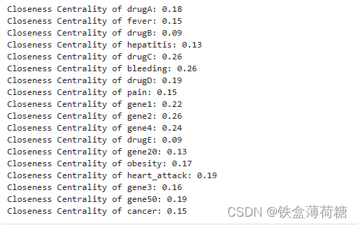
Closeness centrality 量化一个节点到达图中所有其他节点的速度。具有较高接近中心性的节点被认为更具中心性，因为它们可以更有效地与其他节点进行通信。

 closeness_centrality = nx.closeness_centrality(G)
 for node, centrality in closeness_centrality.items():
     print(f'Closeness Centrality of {node}: {centrality:.2f}')

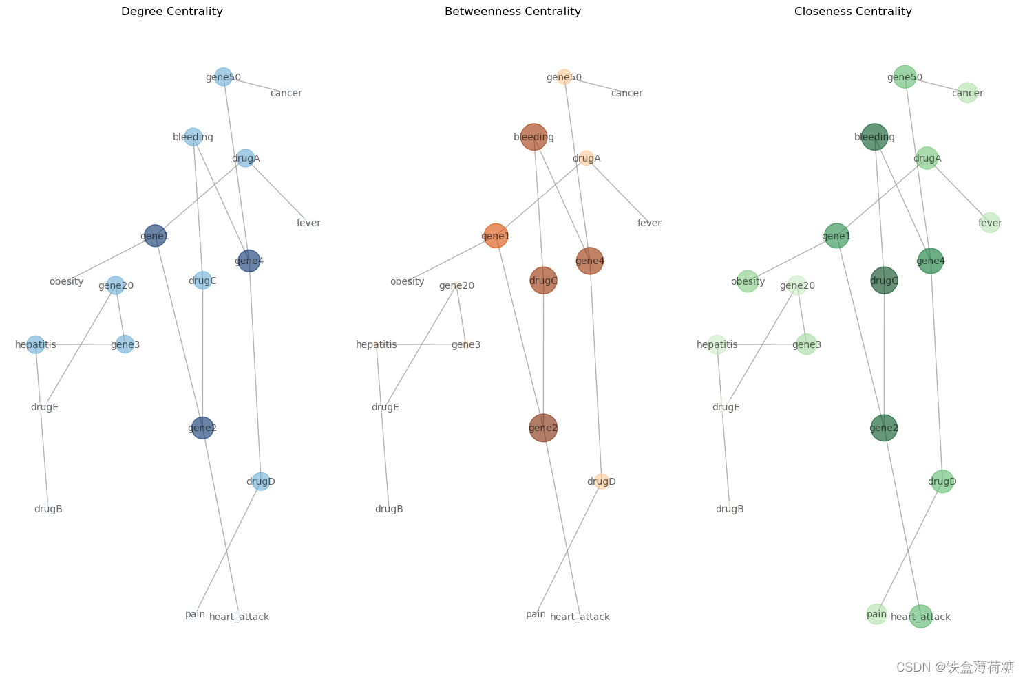
（3）将上述节点中心性分析进行可视化

 # Calculate centrality measures
 degree_centrality = nx.degree_centrality(G)
 betweenness_centrality = nx.betweenness_centrality(G)
 closeness_centrality = nx.closeness_centrality(G)
 
 # Visualize centrality measures
 plt.figure(figsize=(15, 10))
 
 # Degree centrality
 plt.subplot(131)
 nx.draw(G, pos, with_labels=True, font_size=10, node_size=[v * 3000 for v in degree_centrality.values()], node_color=list(degree_centrality.values()), cmap=plt.cm.Blues, edge_color='gray', alpha=0.6)
 plt.title('Degree Centrality')
 
 # Betweenness centrality
 plt.subplot(132)
 nx.draw(G, pos, with_labels=True, font_size=10, node_size=[v * 3000 for v in betweenness_centrality.values()], node_color=list(betweenness_centrality.values()), cmap=plt.cm.Oranges, edge_color='gray', alpha=0.6)
 plt.title('Betweenness Centrality')
 
 # Closeness centrality
 plt.subplot(133)
 nx.draw(G, pos, with_labels=True, font_size=10, node_size=[v * 3000 for v in closeness_centrality.values()], node_color=list(closeness_centrality.values()), cmap=plt.cm.Greens, edge_color='gray', alpha=0.6)
 plt.title('Closeness Centrality')
 
 plt.tight_layout()
 plt.show()

（4）最短路径分析

 最短路径分析的重点是寻找图中两个节点之间的最短路径。这可以帮助理解不同实体之间的连通性，以及连接它们所需的最小关系数量。例如，假设你想找到节点“gene2”和“cancer”之间的最短路径：

 source_node = 'gene2'
 target_node = 'cancer'
 
 # Find the shortest path
 shortest_path = nx.shortest_path(G, source=source_node, target=target_node)
 
 # Visualize the shortest path
plt.figure(figsize=(10, 8))
path_edges = [(shortest_path[i], shortest_path[i + 1]) for i in range(len(shortest_path) - 1)]
nx.draw(G, pos, with_labels=True, font_size=10, node_size=700, node_color='lightblue', edge_color='gray', alpha=0.6)
nx.draw_networkx_edges(G, pos, edgelist=path_edges, edge_color='red', width=2)
plt.title(f'Shortest Path from {source_node} to {target_node}')
plt.show()
print('Shortest Path:', shortest_path)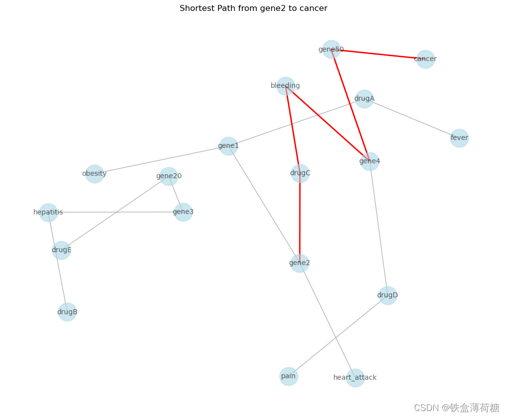

 源节点“gene2”和目标节点“cancer”之间的最短路径用红色突出显示，整个图的节点和边缘也被显示出来。

5.图嵌入（暂时用不到，不学习，有需要的可以去看原链接）

图嵌入是连续向量空间中图中节点或边的数学表示。这些嵌入捕获图的结构和关系信息，允许我们执行各种分析，例如节点相似性计算和在低维空间中的可视化。

 （1）使用node2vec算法，该算法通过在图上执行随机游走并优化以保留节点的局部邻域结构来学习嵌入。

需要下载node2vec库

pip install node2vec