PointNet代码实现——tensorflow2框架

PointNet代码实现——tensorflow2框架

前两天读了一下PointNet的论文，看了一下源码是用tensorflow1写的，关于tensorflow2实现PointNet的博客比较少，所以就自己查找资料复现了一下，数据集用的是ModelNet40。

数据集地址(npz格式)：https://www.kaggle.com/datasets/fanzhiyu123/modelnet40

0. 导入相关包

import gc
gc.enable()

import numpy as np

import tensorflow as tf
from tensorflow import keras    
from tensorflow.keras import layers

from matplotlib import pyplot as pl

1. 对GPU进行配置

#对GPU进行配置
gpus = tf.config.experimental.list_physical_devices('GPU')  #查看

for gpu in gpus:
  tf.config.experimental.set_memory_growth(gpu, True)

2.导入数据

doc = np.load('../input/modelnet40/ModelNet40.npz')
N_CLASS = 40 # 和数据类型数量一致

x_train = doc['x_train']
y_train = doc['y_train']

x_test = doc['x_test']
y_test = doc['y_test']

y_train = np.reshape(y_train,(9840,1,40))
y_test = np.reshape(y_test,(2468,1,40))

3.网络结构设计

#卷积块
def conv_block(input_tensor, filters):
    x = tf.keras.layers.Conv1D(filters, kernel_size=1)(input_tensor) #用的1维卷积，滤波器数量为filters，卷积核大的大小为1，实际上卷积大小为kerner_size*input_channels，（ps:Ptorch的Conv1D和tensorflow的实现方式不太一样)
    x = tf.keras.layers.BatchNormalization()(x) #每次卷积后进行批归一化，加速网络的收敛速度
    return tf.keras.layers.ReLU()(x) #增加非线性

#全连接层
def dense_block(input_tensor, units):
    x = tf.keras.layers.Dense(units)(input_tensor) #全连接层，输出维度为units
    x = tf.keras.layers.BatchNormalization()(x) #每次全连接后进行批归一化，加速网络的收敛速度
    return tf.keras.layers.ReLU()(x) #增加非线性

#最后的分类 label prediction
def classification_net(input_tensor, n_classes):
    x = dense_block(input_tensor, 512) #神经元个数为512的全连接层
    x = tf.keras.layers.Dropout(0.3)(x) #Dropout一下防止过拟合，原作者在这里使用了Dropout
    x = dense_block(x, 256) #神经元个数为256的全连接层
    x = tf.keras.layers.Dropout(0.3)(x) #Dropout一下防止过拟合，原作者在这里使用了Dropout
    return tf.keras.layers.Dense(
        n_classes, activation="softmax" #通过softmax进行分类，类数共有n_classes种
    )(x)

#正交规范化
'''
主要通过将权重推向最近的正交流形来鼓励权重的正交
在梯度反向传播时有一定好处，特别是梯度爆炸和梯度消散的情况，不变会有助于梯度爆炸或梯度消散
'''
class OrthogonalRegularizer(tf.keras.regularizers.Regularizer):
        
    def __init__(self, num_features, l2=0.001):
        self.num_features = num_features
        self.l2 = l2 #l2正则化
        self.I = tf.eye(num_features) #创建大小为num_features的方形单位矩阵
    #计算正交化后的结果
    def __call__(self, inputs):
        A = tf.reshape(inputs, (-1, self.num_features, self.num_features)) 
        AAT = tf.tensordot(A, A, axes=(2, 2))
        AAT = tf.reshape(AAT, (-1, self.num_features, self.num_features))
        return tf.reduce_sum(self.l2 * tf.square(AAT - self.I))

#TNet网络
'''
为了保证变换下的不变性，作者在提取特征之前，先对点云数据进行对齐。对齐操作是通过训练一个小型的网络（TNet）来得到转换矩阵
T-net，和大网络类似，由点独立特征提取，最大池化和全连接层的基本模块组成
作者的思路应该是经过统一的变换，原本无序的点就相当一变换到了一个统一的空间里
'''
def TNet(input_tensor, num_points, features):
    x = conv_block(input_tensor, 64) #过滤器为64的卷积
    x = conv_block(x, 128) #过滤器为128的卷积
    x = conv_block(x, 1024) #过滤器为1024的卷积
    #以上是通过卷积升维操作
    x = tf.keras.layers.MaxPooling1D(pool_size=num_points)(x) #最大池化，大小变成了 BatchSize*1*1024
    x = dense_block(x, 512) #神经元个数为512的全连接
    x = dense_block(x, 256) #神经元个数为256的全连接
    x = tf.keras.layers.Dense(
        features * features, #个数为features的平方
        kernel_initializer="zeros", #权值初始化为0
        bias_initializer=tf.keras.initializers.Constant(
            tf.reshape(tf.cast(tf.eye(features), dtype=tf.float32), [-1])
        ), #偏差初始化
        activity_regularizer=OrthogonalRegularizer(features) #正交正则化
    )(x) #全连接层，输出大小为Batch_size*1*features的平方
    x = tf.reshape(x, (-1, features, features)) #reshape成（Batch_size,features, features)
    return x

#PointNet分类网络的实现，可以看出来确实网络结构比较简单
def PointNetClassifier(num_points, n_classes):
    
    input_tensor = tf.keras.Input(shape=(num_points, 3))#输入大小为（Batch_size，num_points, 3）
    x_t = TNet(input_tensor, num_points, 3) #通过features个数为3的TNet网络对点云数据进行对齐，输出大小为（Batch_size，3, 3）
    x = tf.matmul(input_tensor, x_t) #将TNet网络输出的结果与未经过TNet网络的数据进行一个相乘的操作，输出大小为（Batch_size，num_points, 3）
    #mlp
    #这里需要注意的提到的MLP均由卷积结构完成
    #比如说将3维映射到64维,其利用64个1x3的卷积核
    x = conv_block(x, 64) #过滤器为64的卷积，输出大小为（Batch_size，num_points, 64）
    x = conv_block(x, 64) #过滤器为64的卷积，输出大小为（Batch_size，num_points, 64）
    x_t = TNet(x, num_points, 64) #通过features个数为64的TNet网络对点云数据进行对齐，输出大小为（Batch_size，64, 64）
    x = tf.matmul(x, x_t) #将TNet网络输出的结果与未经过TNet网络的数据进行一个相乘的操作，输出大小为（Batch_size，num_points, 64）
    #mlp 
    x = conv_block(x, 64)  #过滤器为64的卷积，输出大小为（Batch_size，num_points, 64）
    x = conv_block(x, 128)  #过滤器为128的卷积，输出大小为（Batch_size，num_points, 128）
    x = conv_block(x, 1024) #过滤器为128的卷积，输出大小为（Batch_size，num_points, 1024）
    x = tf.keras.layers.MaxPooling1D(pool_size=num_points)(x)  #最大值池化，针对点云的排列不变性，使用了对称函数，采用maxpooling方法来聚合点集信息，输出大小为（Batch_size，1 , 1024）
    output_tensor = classification_net(x, n_classes) #最后进行分类，输出大小为（Batch_size，1 ,  n_classes）
    return tf.keras.Model(input_tensor, output_tensor) #返回模型

model = PointNetClassifier(2048, N_CLASS) #获取模型，num_points为2048，数据集class为40

# 打印模型
model.summary()

'''
keras.utils.plot_model( model,
                        to_file = 'pointnet.png',
                        show_shapes = True,
                        show_layer_names = True,
                        dpi = 200 )
'''

4.模型编译

model.compile( loss = 'categorical_crossentropy', #交叉熵损失函数
               optimizer = keras.optimizers.Adam(learning_rate=0.001), # 采用Adam优化器，学习率为0.001
               metrics = ['accuracy'] )

5. 绘制图像

class PlotProgress(keras.callbacks.Callback):

    def __init__(self, entity = ['loss', 'accuracy']):
        self.entity = entity

    def on_train_begin(self, logs={}):
        self.i = 0
        self.x = []
        
        self.losses = []
        # self.val_losses = []

        self.accs = []
        self.val_accs = []

        self.logs = []

    def on_epoch_end(self, epoch, logs={}):
        self.logs.append(logs)
        self.x.append(self.i)
        # 损失函数
        self.losses.append(logs.get('{}'.format(self.entity[0])))
        # self.val_losses.append(logs.get('val_{}'.format(self.entity[0])))
        # 准确率
        self.accs.append(logs.get('{}'.format(self.entity[1])))
        self.val_accs.append(logs.get('val_{}'.format(self.entity[1])))

        self.i += 1
        
        plt.figure( figsize = (6, 3) )

        plt.subplot(121)
        plt.plot(self.x, self.losses, label="{}".format(self.entity[0]))
        # plt.plot(self.x, self.val_losses, label="val_{}".format(self.entity[0]))
        plt.legend()
        plt.title('loss')
        plt.grid()

        plt.subplot(122)
        plt.plot(self.x, self.accs, label="{}".format(self.entity[1]))
        plt.plot(self.x, self.val_accs, label="val_{}".format(self.entity[1]))
        plt.legend()
        plt.title('accuracy')
        plt.grid()

        plt.tight_layout() # 减少白边
        plt.savefig('visualization@ModelNet40.png')
        plt.close() # 关闭

# 绘图函数
plot_progress = PlotProgress(entity = ['loss', 'accuracy'])

# 早产
from tensorflow.keras.callbacks import EarlyStopping
early_stopping = EarlyStopping( monitor = 'val_accuracy',
                                patience = 20,
                                restore_best_weights = True )

6.模型训练

model.fit( x_train, y_train,
           validation_data = (x_test, y_test),
           
           epochs = 10000, batch_size = 32,

           callbacks = [plot_progress, early_stopping],

           # max_queue_size = 16,
           workers = 8, # 多进程核心数
           use_multiprocessing = True, # 多进程

           shuffle = True, # 再次打乱
           verbose = 1, # 2 一次一行 1 动态进度条
           )
# 只保存验证集准确率最高的那个
model.save_weights('pointnet_weights@ModelNet40.h5')

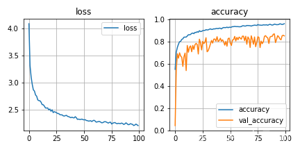
7.训练结果

最后训练了100个epoch，结果如下：