


文章目录
- 65.直角坐标系图表的通用方法
- 66.Boxplot:箱形图
- 66.1 Boxplot - Boxplot_light_velocity
- 66.2 Boxplot - Boxplot_base
- ?66.3 Boxplot - Multiple_categories
- 66.4 Season:Boxplot-grid()返回的对象,可以嵌套在page.add()中。
- 66.5 Season:Boxplot的prepare_data(items)函数
- 66.6 Season:Boxplot的实践-Boxplot_light_velocity()
- 67.EffectScatter:涟漪特效散点图
- 67.1 Effectscatter - Effectscatter_symbol
- 67.2 Effectscatter - Effectscatter_base
- 67.3 Effectscatter - Effectscatter_splitline
- 68.HeatMap:热力图
- 68.1 Heatmap - Heatmap_with_label_show
- 68.2 Heatmap - Heatmap_on_cartesian
- 68.3 Heatmap - Heatmap_base
- 68.4 Sesaon:Heatmap实践-利用pandas和openpyxl预处理数据,一键生成pyecharts要的数据。
- 69.Kline/Candlestick:K线图
- ?69.1 Candlestick - Professional_kline_chart
- 69.2 Candlestick - Kline_itemstyle
- 69.3 Candlestick - Basic_candlestick
- 69.4 Candlestick - Kline_markline
- 69.5 Candlestick - Kline_base
- 69.6 Candlestick - Kline_datazoom_inside
- 69.7 Candlestick - Kline_datazoom_slider_position
- ?69.8 Candlestick - Professional_kline_brush
- 69.9 Candlestick - Kline_datazoom_slider
- 69.10 Candlestick - Kline_split_area
- 69.11 Season实践:Candlestick--yaxis_opts=opts.AxisOpts(is_scale=True)
- 70.Line:折线/面积图
- 70.1 Line - Temperature_change_line_chart
- 70.2 Line - Line_areastyle_boundary_gap
- 70.3 Line - Basic_line_chart
- 70.4 Line - Line_connect_null
- 70.5 Line - Log_axis
- 70.6 Line - Stacked_line_chart
- 70.7 Line - Line_base
- 70.8 Line - Line_yaxis_log
- ?70.9 Line - Rainfall_and_water_flow
- 70.10 Line - Basic_area_chart
- 70.12 Line - Line_smooth
- ?70.13 Line - Multiple_x_axes
- 70.14 Line - Stacked_area_chart
- 70.15 Line - Line_step
- ?70.16 Line - Line_color_with_js_func
- 70.17 Line - Smoothed_line_chart
- 70.18 Line - Line_markpoint_custom
- 70.19 Line - Distribution_of_electricity
- ?70.20 Line - Beautiful_line_chart
- ?70.21 Line - Beijing_aqi(难)
- 70.22 Line - Line_style_and_item_style
- 70.23 Line - Line_markpoint
- 70.24 Line - Line_markline
- 70.25 Line - Line_itemstyle
- 70.26 Line - Line_area_style
- 70.27 Season实践:Line运用pieces设定不同时期的颜色
- 71.PictorialBar:象形柱状图
- 71.1 Pictorialbar - Pictorialbar_base
- 71.2 Pictorialbar - Pictorialbar_multi_custom_symbols
- 71.3 Pictorialbar - Pictorialbar_custom_symbol
- 71.4 Season实践:PictorialBar-自定义图例
- 71.5 Season实践:PictorialBar-自定义图例2
- 72.Scatter:散点图
- 72.1 Scatter - Basic_scatter_chart
- 72.2 Scatter - Scatter_multi_dimension
- 72.3 Scatter - Scatter_visualmap_color
- 72.4 Scatter - Scatter_splitline
- 72.5 Scatter - Scatter_visualmap_size
- 72.6 Season实践:VisualMapOpts(type_: str = "color","size")
- 73.Overlap:层叠多图
- 73.1 Overlap - Overlap_bar_line
- 73.2 Overlap - Overlap_line_scatter
65.直角坐标系图表的通用方法
- 直角坐标系图表继承自 RectChart 都拥有以下方法。
- func RectChart.extend_axis 扩展 X/Y 轴
def extend_axis(
    # 扩展 X 坐标轴数据项
    xaxis_data: Sequence = None,

    # 扩展 X 坐标轴配置项,参考 `global_options.AxisOpts`
    xaxis: Union[opts.AxisOpts, dict, None] = None,

    # 新增 Y 坐标轴配置项,参考 `global_options.AxisOpts`
    yaxis: Union[opts.AxisOpts, dict, None] = None,
)
- func RectChart.add_xaxis 新增 X 轴数据
def add_xaxis(
    # X 轴数据项
    xaxis_data: Sequence
)
- func RectChart.reversal_axis 翻转 XY 轴数据
def reversal_axis():
- func RectChart.overlap 层叠多图
def overlap(
    # chart 为直角坐标系类型图表
    chart: Base
)
- func Chart.add_dataset
def add_dataset(
    # 原始数据。一般来说,原始数据表达的是二维表。
    source: types.Union[types.Sequence, types.JSFunc] = None,

    # 使用 dimensions 定义 series.data 或者 dataset.source 的每个维度的信息。
    dimensions: types.Optional[types.Sequence] = None,

    # dataset.source 第一行/列是否是 维度名 信息。可选值:
    # null/undefine(对应 Python 的 None 值):默认,自动探测。
    # true:第一行/列是维度名信息。
    # false:第一行/列直接开始是数据。
    source_header: types.Optional[bool] = None,
)
66.Boxplot:箱形图
- class pyecharts.charts.Boxplot(RectChart)
class Boxplot(
    # 初始化配置项,参考 `global_options.InitOpts`
    init_opts: opts.InitOpts = opts.InitOpts()
)
- func pyecharts.charts.Boxplot.add_yaxis
def add_yaxis(
    # 系列名称,用于 tooltip 的显示,legend 的图例筛选。
    series_name: str,

    # 系列数据
    y_axis: types.Sequence[types.Union[opts.BoxplotItem, dict]],

    # 是否选中图例
    is_selected: bool = True,

    # 使用的 x 轴的 index,在单个图表实例中存在多个 x 轴的时候有用。
    xaxis_index: Optional[Numeric] = None,

    # 使用的 y 轴的 index,在单个图表实例中存在多个 y 轴的时候有用。
    yaxis_index: Optional[Numeric] = None,

    # 标签配置项,参考 `series_options.LabelOpts`
    label_opts: Union[opts.LabelOpts, dict] = opts.LabelOpts(),

    # 标记点配置项,参考 `series_options.MarkPointOpts`
    markpoint_opts: Union[opts.MarkPointOpts, dict] = opts.MarkPointOpts(),

    # 标记线配置项,参考 `series_options.MarkLineOpts`
    markline_opts: Union[opts.MarkLineOpts, dict] = opts.MarkLineOpts(),

    # 提示框组件配置项,参考 `series_options.TooltipOpts`
    tooltip_opts: Union[opts.TooltipOpts, dict, None] = None,

    # 图元样式配置项,参考 `series_options.ItemStyleOpts`
    itemstyle_opts: Union[opts.ItemStyleOpts, dict, None] = None,
)
- BoxplotItem:箱形图数据项
class BoxplotItem(
    # 数据项名称。
    name: Optional[str] = None,

    # 单个数据项的数值。
    value: Optional[Numeric] = None,

    # 文本的样式设置,参考 `series_options.LabelOpts`。
    label_opts: Union[LabelOpts, dict, None] = None,

    # 图元样式配置项,参考 `series_options.ItemStyleOpts`
    itemstyle_opts: Union[ItemStyleOpts, dict, None] = None,

    # 提示框组件配置项,参考 `series_options.TooltipOpts`
    tooltip_opts: Union[TooltipOpts, dict, None] = None,
)
- boyplot.py
class Boxplot(RectChart):
    """
    <<< Boxplot >>>

    A box-plot is a statistical chart used to show a set of data dispersion data.
    It displays the maximum, minimum, median, lower quartile, and upper quartile
    of a set of data.
    """

    def add_yaxis(
        self,
        series_name: str,
        y_axis: types.Sequence[types.Union[opts.BoxplotItem, dict]],
        *,
        is_selected: bool = True,
        xaxis_index: types.Optional[types.Numeric] = None,
        yaxis_index: types.Optional[types.Numeric] = None,
        label_opts: types.Label = opts.LabelOpts(),
        markpoint_opts: types.MarkPoint = opts.MarkPointOpts(),
        markline_opts: types.MarkLine = opts.MarkLineOpts(),
        tooltip_opts: types.Tooltip = None,
        itemstyle_opts: types.ItemStyle = None,
    ):
        self._append_legend(series_name, is_selected)
        self.options.get("series").append(
            {
                "type": ChartType.BOXPLOT,
                "name": series_name,
                "xAxisIndex": xaxis_index,
                "yAxisIndex": yaxis_index,
                "data": y_axis,
                "label": label_opts,
                "markPoint": markpoint_opts,
                "markLine": markline_opts,
                "tooltip": tooltip_opts,
                "itemStyle": itemstyle_opts,
            }
        )
        return self

    @staticmethod
    def prepare_data(items):
        data = []
        for item in items:
            try:
                d, res = sorted(item), []
                for i in range(1, 4):
                    n = i * (len(d) + 1) / 4
                    k = int(n)
                    m = n - k
                    if m == 0:
                        res.append(d[k - 1])
                    elif m == 1 / 4:
                        res.append(d[k - 1] * 0.75 + d[k] * 0.25)
                    elif m == 1 / 2:
                        res.append(d[k - 1] * 0.50 + d[k] * 0.50)
                    elif m == 3 / 4:
                        res.append(d[k - 1] * 0.25 + d[k] * 0.75)
                data.append([d[0]] + res + [d[-1]])
            except Exception:
                pass
        return data
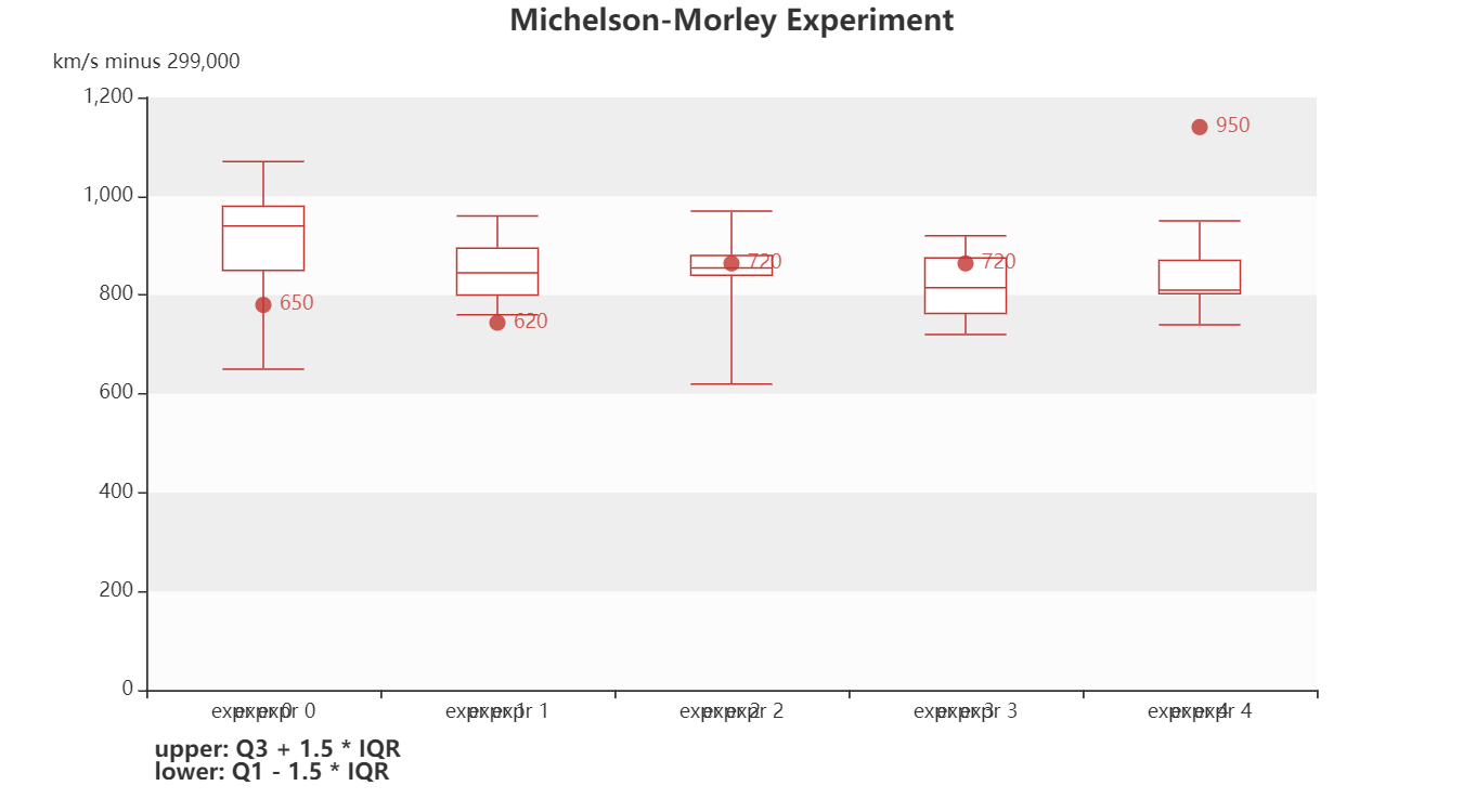
66.1 Boxplot - Boxplot_light_velocity
import pyecharts.options as opts
from pyecharts.charts import Grid, Boxplot, Scatter


y_data = [
    [
        850,
        740,
        900,
        1070,
        930,
        850,
        950,
        980,
        980,
        880,
        1000,
        980,
        930,
        650,
        760,
        810,
        1000,
        1000,
        960,
        960,
    ],
    [
        960,
        940,
        960,
        940,
        880,
        800,
        850,
        880,
        900,
        840,
        830,
        790,
        810,
        880,
        880,
        830,
        800,
        790,
        760,
        800,
    ],
    [
        880,
        880,
        880,
        860,
        720,
        720,
        620,
        860,
        970,
        950,
        880,
        910,
        850,
        870,
        840,
        840,
        850,
        840,
        840,
        840,
    ],
    [
        890,
        810,
        810,
        820,
        800,
        770,
        760,
        740,
        750,
        760,
        910,
        920,
        890,
        860,
        880,
        720,
        840,
        850,
        850,
        780,
    ],
    [
        890,
        840,
        780,
        810,
        760,
        810,
        790,
        810,
        820,
        850,
        870,
        870,
        810,
        740,
        810,
        940,
        950,
        800,
        810,
        870,
    ],
]
scatter_data = [650, 620, 720, 720, 950, 970]

box_plot = Boxplot()

box_plot = (
    box_plot.add_xaxis(xaxis_data=["expr 0", "expr 1", "expr 2", "expr 3", "expr 4"])
    .add_yaxis(series_name="", y_axis=box_plot.prepare_data(y_data))
    .set_global_opts(
        title_opts=opts.TitleOpts(
            pos_left="center", title="Michelson-Morley Experiment"
        ),
        tooltip_opts=opts.TooltipOpts(trigger="item", axis_pointer_type="shadow"),
        xaxis_opts=opts.AxisOpts(
            type_="category",
            boundary_gap=True,
            splitarea_opts=opts.SplitAreaOpts(is_show=False),
            axislabel_opts=opts.LabelOpts(formatter="expr {value}"),
            splitline_opts=opts.SplitLineOpts(is_show=False),
        ),
        yaxis_opts=opts.AxisOpts(
            type_="value",
            name="km/s minus 299,000",
            splitarea_opts=opts.SplitAreaOpts(
                is_show=True, areastyle_opts=opts.AreaStyleOpts(opacity=1)
            ),
        ),
    )
    .set_series_opts(tooltip_opts=opts.TooltipOpts(formatter="{b}: {c}"))
)

scatter = (
    Scatter()
    .add_xaxis(xaxis_data=["expr 0", "expr 1", "expr 2", "expr 3", "expr 4"])
    .add_yaxis(series_name="", y_axis=scatter_data)
    .set_global_opts(
        title_opts=opts.TitleOpts(
            pos_left="10%",
            pos_top="90%",
            title="upper: Q3 + 1.5 * IQR \nlower: Q1 - 1.5 * IQR",
            title_textstyle_opts=opts.TextStyleOpts(
                border_color="#999", border_width=1, font_size=14
            ),
        ),
        yaxis_opts=opts.AxisOpts(
            axislabel_opts=opts.LabelOpts(is_show=False),
            axistick_opts=opts.AxisTickOpts(is_show=False),
        ),
    )
)

grid = (
    Grid(init_opts=opts.InitOpts(width="1600px", height="1000px"))
    .add(
        box_plot,
        grid_opts=opts.GridOpts(pos_left="10%", pos_right="10%", pos_bottom="15%"),
    )
    .add(
        scatter,
        grid_opts=opts.GridOpts(pos_left="10%", pos_right="10%", pos_bottom="15%"),
    )
    .render("boxplot_light_velocity.html")
)
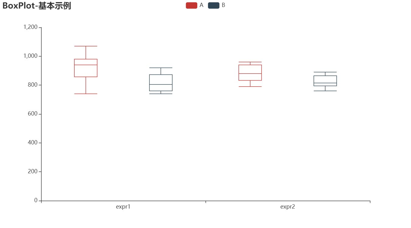
66.2 Boxplot - Boxplot_base
from pyecharts import options as opts
from pyecharts.charts import Boxplot

v1 = [
    [850, 740, 900, 1070, 930, 850, 950, 980, 980, 880, 1000, 980],
    [960, 940, 960, 940, 880, 800, 850, 880, 900, 840, 830, 790],
]
v2 = [
    [890, 810, 810, 820, 800, 770, 760, 740, 750, 760, 910, 920],
    [890, 840, 780, 810, 760, 810, 790, 810, 820, 850, 870, 870],
]
c = Boxplot()
c.add_xaxis(["expr1", "expr2"])
c.add_yaxis("A", c.prepare_data(v1))
c.add_yaxis("B", c.prepare_data(v2))
c.set_global_opts(title_opts=opts.TitleOpts(title="BoxPlot-基本示例"))
c.render("boxplot_base.html")
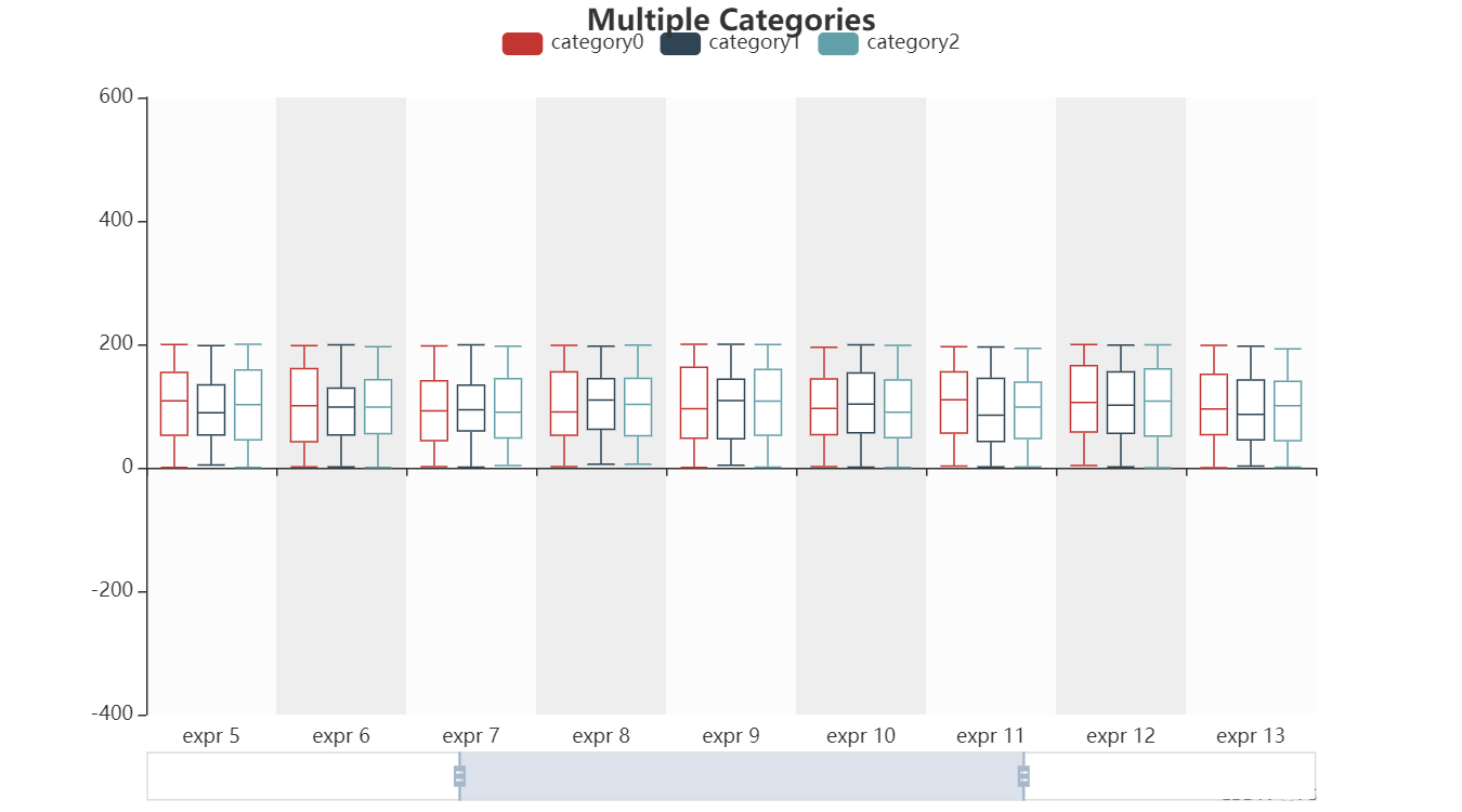
?66.3 Boxplot - Multiple_categories
import pyecharts.options as opts
from pyecharts.charts import Boxplot
from pyecharts.commons.utils import JsCode
axis_data = [
"0",
"1",
"2",
"3",
"4",
"5",
"6",
"7",
"8",
"9",
"10",
"11",
"12",
"13",
"14",
"15",
"16",
"17",
]
data = [
{
"axisData": axis_data,
"boxData": [
[
3.8888578346043534,
55.82692798765428,
98.71608835477272,
149.50917642877687,
196.31621070646452,
],
[
0.5174326704765253,
47.52990128406776,
103.66600287106233,
160.1380046605997,
194.8294269298398,
],
[
2.843900448603165,
51.773788199388605,
90.66830693679475,
152.19938074181786,
196.18172012742428,
],
[
2.6752702891334135,
42.85051429480143,
98.54433643572133,
166.81852013033875,
199.7400516615198,
],
[
1.665511467481906,
63.069856326089585,
123.20638438572043,
164.0932194814393,
199.56631692214057,
],
[
0.3597414263118992,
52.84424125860876,
108.14491539985673,
154.42390255012828,
199.39872381823812,
],
[
1.3380322954592128,
41.989379994726335,
100.39118095266713,
160.38742881881478,
197.8251968350275,
],
[
1.7005873932608662,
43.88170786936796,
92.29415890464293,
140.7858956683471,
197.50510824352313,
],
[
1.7017445023542965,
52.55872982785781,
90.26972335102536,
155.43082163069883,
198.31679368721197,
],
[
0.45657888665799895,
47.60747957375436,
95.53917053451289,
162.55256484073354,
199.78317232079928,
],
[
1.745438082254136,
53.450845301261964,
95.8847297380051,
143.99885640751006,
195.1863502057908,
],
[
2.5631287114048273,
56.04486879215165,
110.01592256847306,
155.33508398386462,
195.90291395560985,
],
[
3.4380745785991262,
58.07888602010247,
105.64925213947652,
165.50126442985191,
199.75877487248675,
],
[
0.03322930419802361,
53.363159200883985,
95.32936635574816,
151.39772626598614,
198.20394907387762,
],
[
0.7063564158257929,
73.89369564248534,
116.6947935806626,
152.93983211466667,
197.1481400480321,
],
[
0.9611585600880268,
46.64283650085793,
102.32004406296502,
148.64094149067978,
199.59803470854715,
],
[
1.4310036755643463,
50.15631363530299,
102.68128938225942,
147.52573154872948,
197.6018158750086,
],
[
0.492994684970105,
43.23619663302313,
99.60815322547333,
140.00299600143438,
198.97693156537883,
],
],
"outliers": [],
},
{
"axisData": axis_data,
"boxData": [
[
1.3866777918670525,
52.723984144413805,
112.16068484025186,
148.07060013196633,
196.6493886555634,
],
[
0.8675025485252785,
41.94008605353009,
90.4944101654473,
134.34314089904032,
199.57411732908722,
],
[
2.109917782227244,
47.361245156921306,
98.03121935506474,
152.57304498745683,
199.6655667235125,
],
[
0.835914742081334,
45.90386054869363,
110.8008994981315,
153.77050147012113,
198.17687983907325,
],
[
0.09929780808608513,
55.313979741487245,
80.36049651385588,
144.5076321261422,
198.71007594348265,
],
[
4.3591904343687204,
53.098201381124454,
88.8716562277704,
134.2243571501588,
197.86166497124387,
],
[
1.4751642002043486,
52.87727910767818,
98.1167484613283,
129.123794134296,
199.26128215126036,
],
[
1.0208468961246275,
59.72883452828452,
93.7117188714775,
133.6955646934541,
199.04002574913483,
],
[
5.700580454086168,
62.30214699943758,
109.4858546359291,
144.37435834128183,
196.80025087232633,
],
[
3.8776389962399627,
47.07485197991684,
108.77911010272065,
143.55929331063112,
199.78963194031576,
],
[
0.9206486824532956,
56.531536633466786,
103.22722183226676,
153.71850265606832,
199.26707930050713,
],
[
1.2238397462105866,
42.37213742602606,
85.0161099008823,
144.6618761115177,
195.68883739488717,
],
[
1.383845313528731,
55.58975449585246,
101.2502031542653,
155.4651069256266,
198.51896538541257,
],
[
2.460600698918336,
45.35279677561122,
86.22855211501036,
142.2985968944624,
196.88095181245973,
],
[
1.5771786133238486,
47.74919144071982,
98.25948642595273,
143.6080569193598,
199.35657813436302,
],
[
1.679597195618454,
54.03099324959242,
93.24925248108138,
156.2197398880975,
199.96087190538344,
],
[
0.09445769268561222,
62.987289799985746,
93.5536375308287,
146.10299624484736,
198.89381360902073,
],
[
0.5074418255246016,
43.16902467382945,
97.5036007943674,
150.07249687988744,
197.1438186145631,
],
],
"outliers": [],
},
{
"axisData": axis_data,
"boxData": [
[
0.17336583192690824,
38.89251480694969,
95.24827036951726,
144.42455874548153,
199.4034309165705,
],
[
3.676663641014155,
56.915752270243615,
116.52533365244228,
154.9613826361874,
199.45242610474344,
],
[
0.2637149176087039,
39.10809721270764,
83.11646124189903,
145.85305644883107,
199.4425993969723,
],
[
0.9435517891188017,
59.34726771939571,
116.9100457332774,
154.6830501745436,
197.360203327316,
],
[
3.979089227580568,
59.55958857930115,
106.50956069508263,
154.19233153204274,
198.27863048295953,
],
[
0.2254389425328185,
45.14272916122666,
101.99744565544017,
158.20585382578935,
199.87918467096276,
],
[
0.4981747166813655,
55.07500323828029,
98.06775843874871,
142.6740673515219,
196.17733451641203,
],
[
3.459413844168191,
48.45434370508197,
90.08287035261958,
144.44636703035508,
196.7330418635301,
],
[
5.491046107788211,
51.726853187011294,
102.73451029578627,
144.81711164442441,
198.8867176824325,
],
[
0.7550472434538769,
52.51096431201062,
107.88318214869264,
159.26961432919137,
199.61830476130777,
],
[
0.2752001848587593,
48.7398963427885,
89.75616732426943,
142.05594236584855,
198.3147751483816,
],
[
1.4946063684317945,
47.50894653631401,
98.11186814575922,
138.51943571666908,
193.3052139732351,
],
[
0.20882224269564986,
51.28631550804623,
107.81597798598389,
160.02354609263347,
199.2878557923929,
],
[
0.8976637474841898,
43.66029575375894,
100.62231619788403,
139.9661197041632,
192.54845617677,
],
[
5.859745717489284,
47.03805156535355,
108.41470873842098,
157.096784096105,
199.9179863824041,
],
[
3.7257707586363598,
42.231249941095996,
97.356821000705,
142.79191220154834,
198.84036692134,
],
[
1.8454208635465985,
44.91333687646406,
98.65350096972611,
143.39018022926803,
199.87483964263296,
],
[
0.5514923538800787,
45.85216189462081,
99.9806157446917,
153.32082407525542,
198.2776454910153,
],
],
"outliers": [],
},
{
"axisData": axis_data,
"boxData": [
[
0.7168805200240325,
46.53681449735687,
97.29254353668016,
156.63006806530143,
199.3015739378797,
],
[
1.7193486665883828,
62.95172603462959,
112.02740143118092,
156.0538383864632,
199.26142301676774,
],
[
2.1369256823901672,
57.21732276358834,
103.36834727083514,
153.72092303549277,
198.79539179393552,
],
[
0.032880351113817596,
47.562260234793726,
96.26764103515997,
145.73458375286407,
199.06617414977254,
],
[
0.4401537603581307,
43.865273442582165,
94.93675834281308,
146.35738146359748,
193.64127816517245,
],
[
0.3961689590249673,
50.96909350725202,
104.73604524329194,
148.23414082526403,
198.8856874527377,
],
[
0.21937305368529003,
49.59183574690416,
102.85949468466653,
163.6266324963084,
199.69745130954797,
],
[
0.6248639849676607,
43.65587924550377,
98.38900488209111,
152.00850019757138,
197.66849547068205,
],
[
0.8836653304501674,
51.715354680095054,
106.27634207918453,
152.75520182409605,
198.7026018674421,
],
[
7.037170236614809,
60.499053468218285,
99.70265208133726,
145.547153860169,
197.56589704383606,
],
[
0.191005947981715,
36.77501191389064,
78.79138996882105,
138.31773623910374,
199.5549011391389,
],
[
2.085660638228548,
50.85562917320624,
100.31437027035244,
144.07227532917557,
199.9671689855977,
],
[
2.8329465269889997,
46.64735576556238,
95.58042897665536,
150.95016495791145,
199.01002263253537,
],
[
2.9140730838620232,
55.8981643150491,
99.12490122897461,
138.35381332244458,
197.89764340001602,
],
[
0.6900722343886834,
61.20627193426343,
108.73896996351209,
152.38197094149575,
199.49695739258172,
],
[
0.3519848056308117,
51.38799178079926,
108.74191700174138,
146.60812022274987,
198.09008264810322,
],
[
0.2761553645218129,
56.388967149570455,
104.8697135719724,
153.5049030271958,
199.5731857965878,
],
[
3.5557869592812708,
46.14828237062535,
108.66363220203428,
160.07663258712037,
199.1028921688903,
],
],
"outliers": [],
},
{
"axisData": axis_data,
"boxData": [
[
2.979477505147443,
39.75713406508555,
94.53079422141971,
156.08283690923398,
199.44795240229735,
],
[
2.6484190473881064,
39.93623770385512,
77.27669464380185,
128.4315475425753,
199.56482718369725,
],
[
0.027555734890816197,
57.0338837796717,
108.81399073964846,
148.06814743102228,
199.60110925244555,
],
[
5.095524117378636,
61.306047315630614,
110.93776130670011,
156.1408460056575,
195.24807037634693,
],
[
2.728611345602383,
44.56605304153001,
82.24512299722713,
147.52018338217582,
197.4401254594119,
],
[
3.2844003726598903,
31.22917030540313,
98.82341804522095,
147.37909270120065,
195.31234405750303,
],
[
0.18212434446978065,
59.703454603359305,
103.67261216911498,
144.78603398715182,
197.894221292169,
],
[
2.0723859910971587,
65.62630968779271,
108.08425190082599,
153.04828999176155,
198.71953877580813,
],
[
0.9675695750262392,
52.06976077477188,
106.44774448853506,
153.71491587328123,
199.9367145735771,
],
[
2.5328359424461766,
54.040914797213425,
98.74095548976766,
156.68297214273787,
199.54362057796757,
],
[
1.1331529861684952,
44.39864814947693,
88.34657630798353,
137.22778263394855,
198.83623456218217,
],
[
0.03400372259445561,
39.0412178839992,
82.44989003395962,
142.39781316172628,
198.66240858068616,
],
[
3.3739669830866514,
51.553716623716575,
113.01026058884891,
165.92964939460416,
198.22988431223231,
],
[
1.7144280578984095,
52.52972703008254,
97.47299182400204,
134.9644807802092,
198.46967348342878,
],
[
1.7893968468841948,
43.87294943558785,
90.42735899685948,
143.0586276081752,
197.6798595904976,
],
[
4.299131337916773,
50.29192506963852,
104.5869339834448,
163.2705302681331,
199.10157077449355,
],
[
0.6740610620747933,
54.02651804107089,
86.12616850846155,
137.7008290515613,
199.78999859299336,
],
[
0.5370189113081292,
50.44519588101707,
98.08928065026996,
139.8482090057953,
197.20820681141507,
],
],
"outliers": [],
},
]
(
Boxplot(init_opts=opts.InitOpts(width="1600px", height="800px"))
.add_xaxis(xaxis_data=axis_data)
.add_yaxis(
series_name="category0",
y_axis=data[0]["boxData"],
tooltip_opts=opts.TooltipOpts(
formatter=JsCode(
"""function(param) { return [
'Experiment ' + param.name + ': ',
'upper: ' + param.data[0],
'Q1: ' + param.data[1],
'median: ' + param.data[2],
'Q3: ' + param.data[3],
'lower: ' + param.data[4]
].join('<br/>') }"""
)
),
)
.add_yaxis(
series_name="category1",
y_axis=data[1]["boxData"],
tooltip_opts=opts.TooltipOpts(
formatter=JsCode(
"""function(param) { return [
'Experiment ' + param.name + ': ',
'upper: ' + param.data[0],
'Q1: ' + param.data[1],
'median: ' + param.data[2],
'Q3: ' + param.data[3],
'lower: ' + param.data[4]
].join('<br/>') }"""
)
),
)
.add_yaxis(
series_name="category2",
y_axis=data[2]["boxData"],
tooltip_opts=opts.TooltipOpts(
formatter=JsCode(
"""function(param) { return [
'Experiment ' + param.name + ': ',
'upper: ' + param.data[0],
'Q1: ' + param.data[1],
'median: ' + param.data[2],
'Q3: ' + param.data[3],
'lower: ' + param.data[4]
].join('<br/>') }"""
)
),
)
.set_global_opts(
title_opts=opts.TitleOpts(title="Multiple Categories", pos_left="center"),
legend_opts=opts.LegendOpts(pos_top="3%"),
tooltip_opts=opts.TooltipOpts(trigger="item", axis_pointer_type="shadow"),
xaxis_opts=opts.AxisOpts(
name_gap=30,
boundary_gap=True,
splitarea_opts=opts.SplitAreaOpts(
areastyle_opts=opts.AreaStyleOpts(opacity=1)
),
axislabel_opts=opts.LabelOpts(formatter="expr {value}"),
splitline_opts=opts.SplitLineOpts(is_show=False),
),
yaxis_opts=opts.AxisOpts(
type_="value",
min_=-400,
max_=600,
splitarea_opts=opts.SplitAreaOpts(is_show=False),
),
datazoom_opts=[
opts.DataZoomOpts(type_="inside", range_start=0, range_end=20),
opts.DataZoomOpts(type_="slider", xaxis_index=0, is_show=True),
],
)
.render("multiple_categories.html")
)
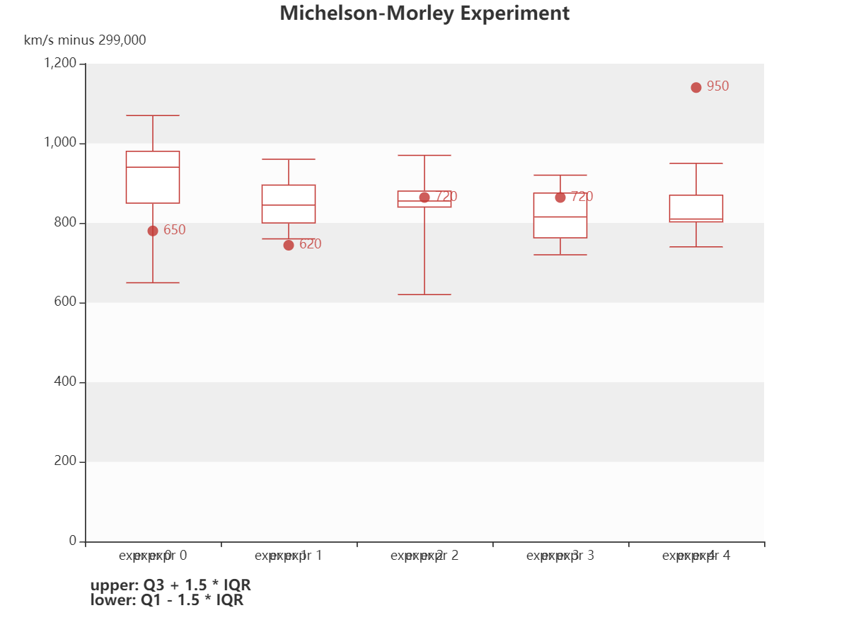
66.4 Season:Boxplot-grid()返回的对象,可以嵌套在page.add()中。
def Boxplot_light_velocity():
    y_data = [
        [850,740,900,1070,930,850,950,980,980,880,1000,980,930,650,760,810,1000,1000,960,960,],
        [960,940,960,940,880,800,850,880,900,840,830,790,810,880,880,830,800,790,760,800,],
        [880,880,880,860,720,720,620,860,970,950,880,910,850,870,840,840,850,840,840,840,],
        [890,810,810,820,800,770,760,740,750,760,910,920,890,860,880,720,840,850,850,780,],
        [890,840,780,810,760,810,790,810,820,850,870,870,810,740,810,940,950,800,810,870,],
    ]
    scatter_data = [650, 620, 720, 720, 950, 970]

    box_plot = Boxplot()

    box_plot = (
        box_plot.add_xaxis(xaxis_data=["expr 0", "expr 1", "expr 2", "expr 3", "expr 4"])
        .add_yaxis(series_name="", y_axis=box_plot.prepare_data(y_data))
        .set_global_opts(
            title_opts=opts.TitleOpts(
                pos_left="center", title="Michelson-Morley Experiment"
            ),
            tooltip_opts=opts.TooltipOpts(trigger="item", axis_pointer_type="shadow"),
            xaxis_opts=opts.AxisOpts(
                type_="category",
                boundary_gap=True,
                splitarea_opts=opts.SplitAreaOpts(is_show=False),
                axislabel_opts=opts.LabelOpts(formatter="expr {value}"),
                splitline_opts=opts.SplitLineOpts(is_show=False),
            ),
            yaxis_opts=opts.AxisOpts(
                type_="value",
                name="km/s minus 299,000",
                splitarea_opts=opts.SplitAreaOpts(
                    is_show=True, areastyle_opts=opts.AreaStyleOpts(opacity=1)
                ),
            ),
        )
        .set_series_opts(tooltip_opts=opts.TooltipOpts(formatter="{b}: {c}"))
    )

    scatter = (
        Scatter()
        .add_xaxis(xaxis_data=["expr 0", "expr 1", "expr 2", "expr 3", "expr 4"])
        .add_yaxis(series_name="", y_axis=scatter_data)
        .set_global_opts(
            title_opts=opts.TitleOpts(
                pos_left="10%",
                pos_top="90%",
                title="upper: Q3 + 1.5 * IQR \nlower: Q1 - 1.5 * IQR",
                title_textstyle_opts=opts.TextStyleOpts(
                    border_color="#999", border_width=1, font_size=14
                ),
            ),
            yaxis_opts=opts.AxisOpts(
                axislabel_opts=opts.LabelOpts(is_show=False),
                axistick_opts=opts.AxisTickOpts(is_show=False),
            ),
        )
    )

    grid = (
        Grid(init_opts=opts.InitOpts(width="800px", height="600px"))
        .add(
            box_plot,
            grid_opts=opts.GridOpts(pos_left="10%", pos_right="10%", pos_bottom="15%"),
        )
        .add(
            scatter,
            grid_opts=opts.GridOpts(pos_left="10%", pos_right="10%", pos_bottom="15%"),
        )
        #.render("boxplot_light_velocity.html")
    )
    return grid
66.5 Season:Boxplot的prepare_data(items)函数
分成最大值、Q75、平均值、Q25、最小值。
    @staticmethod
    def prepare_data(items):
        data = []
        for item in items:
            try:
                d, res = sorted(item), []
                for i in range(1, 4):
                    n = i * (len(d) + 1) / 4
                    k = int(n)
                    m = n - k
                    if m == 0:
                        res.append(d[k - 1])
                    elif m == 1 / 4:
                        res.append(d[k - 1] * 0.75 + d[k] * 0.25)
                    elif m == 1 / 2:
                        res.append(d[k - 1] * 0.50 + d[k] * 0.50)
                    elif m == 3 / 4:
                        res.append(d[k - 1] * 0.25 + d[k] * 0.75)
                data.append([d[0]] + res + [d[-1]])
            except Exception:
                pass
        return data
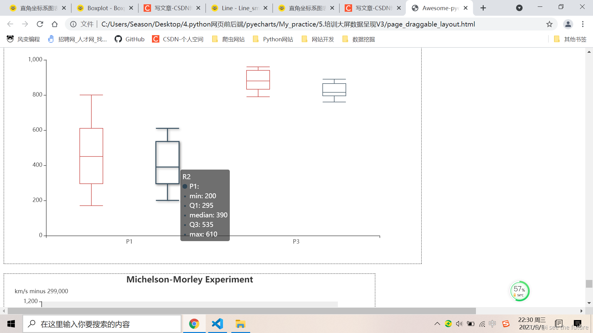
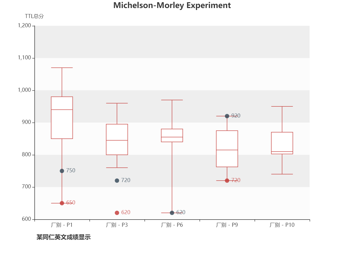
66.6 Season:Boxplot的实践-Boxplot_light_velocity()
def Boxplot_light_velocity():
    y_data = [
        [850,740,900,1070,930,850,950,980,980,880,1000,980,930,650,760,810,1000,1000,960,960,],
        [960,940,960,940,880,800,850,880,900,840,830,790,810,880,880,830,800,790,760,800,],
        [880,880,880,860,720,720,620,860,970,950,880,910,850,870,840,840,850,840,840,840,],
        [890,810,810,820,800,770,760,740,750,760,910,920,890,860,880,720,840,850,850,780,],
        [890,840,780,810,760,810,790,810,820,850,870,870,810,740,810,940,950,800,810,870,],
    ]
    scatter_data = [650, 620, '-', 720, '-']
    scatter_data2 = [750, 720, 620, 920, '-']

    box_plot = Boxplot()

    box_plot = (
        box_plot.add_xaxis(xaxis_data=["P1", "P3", "P6", "P9", "P10"])
        .add_yaxis(series_name="", y_axis=box_plot.prepare_data(y_data))
        .set_global_opts(
            title_opts=opts.TitleOpts(
                pos_left="center", title="Michelson-Morley Experiment"
            ),
            tooltip_opts=opts.TooltipOpts(trigger="item", axis_pointer_type="shadow"),
            xaxis_opts=opts.AxisOpts(
                type_="category",
                boundary_gap=True,
                splitarea_opts=opts.SplitAreaOpts(is_show=False),
                axislabel_opts=opts.LabelOpts(formatter="厂别 - {value}"),
                splitline_opts=opts.SplitLineOpts(is_show=False),
            ),
            yaxis_opts=opts.AxisOpts(
                type_="value",
                name="TTL总分",
                splitarea_opts=opts.SplitAreaOpts(
                    is_show=True, areastyle_opts=opts.AreaStyleOpts(opacity=1)
                ),
                min_="600",
                max_="1200",
            ),
        )
        .set_series_opts(tooltip_opts=opts.TooltipOpts(formatter="{b}: {c}"))
    )

    scatter = (
        Scatter()
        .add_xaxis(xaxis_data=[])
        .add_yaxis(series_name="", y_axis=scatter_data)
        .add_yaxis(series_name="", y_axis=scatter_data2)
        .set_global_opts(
            title_opts=opts.TitleOpts(
                pos_left="10%",
                pos_top="90%",
                title="某同仁英文成绩显示",
                title_textstyle_opts=opts.TextStyleOpts(
                    border_color="#999", border_width=1, font_size=14
                ),
            ),
            yaxis_opts=opts.AxisOpts(
                axislabel_opts=opts.LabelOpts(is_show=False),
                axistick_opts=opts.AxisTickOpts(is_show=False),
                min_="600",
                max_="1200",
            ),
        )
    )

    grid = (
        Grid(init_opts=opts.InitOpts(width="800px", height="600px"))
        .add(
            box_plot,
            grid_opts=opts.GridOpts(pos_left="10%", pos_right="10%", pos_bottom="15%"),
        )
        .add(
            scatter,
            grid_opts=opts.GridOpts(pos_left="10%", pos_right="10%", pos_bottom="15%"),
        )
        #.render("boxplot_light_velocity.html")
    )
    return grid
67.EffectScatter:涟漪特效散点图
- class pyecharts.charts.EffectScatter(RectChart)
class EffectScatter(
    # 初始化配置项,参考 `global_options.InitOpts`
    init_opts: opts.InitOpts = opts.InitOpts()
)
- func pyecharts.charts.EffectScatter.add_yaxis
 def add_yaxis(
     # 系列名称,用于 tooltip 的显示,legend 的图例筛选。
    series_name: str,

    # 系列数据
    y_axis: types.Sequence[types.Union[opts.BoxplotItem, dict]],

    # 是否选中图例
    is_selected: bool = True,

    # 使用的 x 轴的 index,在单个图表实例中存在多个 x 轴的时候有用。
    xaxis_index: Optional[Numeric] = None,

    # 使用的 y 轴的 index,在单个图表实例中存在多个 y 轴的时候有用。
    yaxis_index: Optional[Numeric] = None,

    # 系列 label 颜色
    color: Optional[str] = None,

    # 标记图形形状
    symbol: Optional[str] = None,

    # 标记的大小
    symbol_size: Numeric = 10,

    # 标记的旋转角度。注意在 markLine 中当 symbol 为 'arrow' 时会忽略 symbolRotate 强制设置为切线的角度。
    symbol_rotate: types.Optional[types.Numeric] = None,

    # 标签配置项,参考 `series_options.LabelOpts`
    label_opts: Union[opts.LabelOpts, dict] = opts.LabelOpts(),

    # 涟漪特效配置项,参考 `series_options.EffectOpts`
    effect_opts: Union[opts.EffectOpts, dict] = opts.EffectOpts(),

    # 提示框组件配置项,参考 `series_options.TooltipOpts`
    tooltip_opts: Union[opts.TooltipOpts, dict, None] = None,

    # 图元样式配置项,参考 `series_options.ItemStyleOpts`
    itemstyle_opts: Union[opts.ItemStyleOpts, dict, None] = None,
)
- EffectScatterItem:涟漪特效散点图数据项
class EffectScatterItem(
    # 数据项名称。
    name: Union[str, Numeric] = None,

    # 数据项的值
    value: Union[str, Numeric] = None,

    # 单个数据标记的图形。
    symbol: Optional[str] = None,

    # 单个数据标记的大小
    symbol_size: Union[Sequence[Numeric], Numeric] = None,

    # 单个数据标记的旋转角度(而非弧度)。
    symbol_rotate: Optional[Numeric] = None,

    # 如果 symbol 是 path:// 的形式,是否在缩放时保持该图形的长宽比。
    symbol_keep_aspect: bool = False,

    # 单个数据标记相对于原本位置的偏移。
    symbol_offset: Optional[Sequence] = None,

    # 标签配置项,参考 `series_options.LabelOpts`
    label_opts: Union[LabelOpts, dict, None] = None,

    # 图元样式配置项,参考 `series_options.ItemStyleOpts`
    itemstyle_opts: Union[ItemStyleOpts, dict, None] = None,

    # 提示框组件配置项,参考 `series_options.TooltipOpts`
    tooltip_opts: Union[TooltipOpts, dict, None] = None,
)
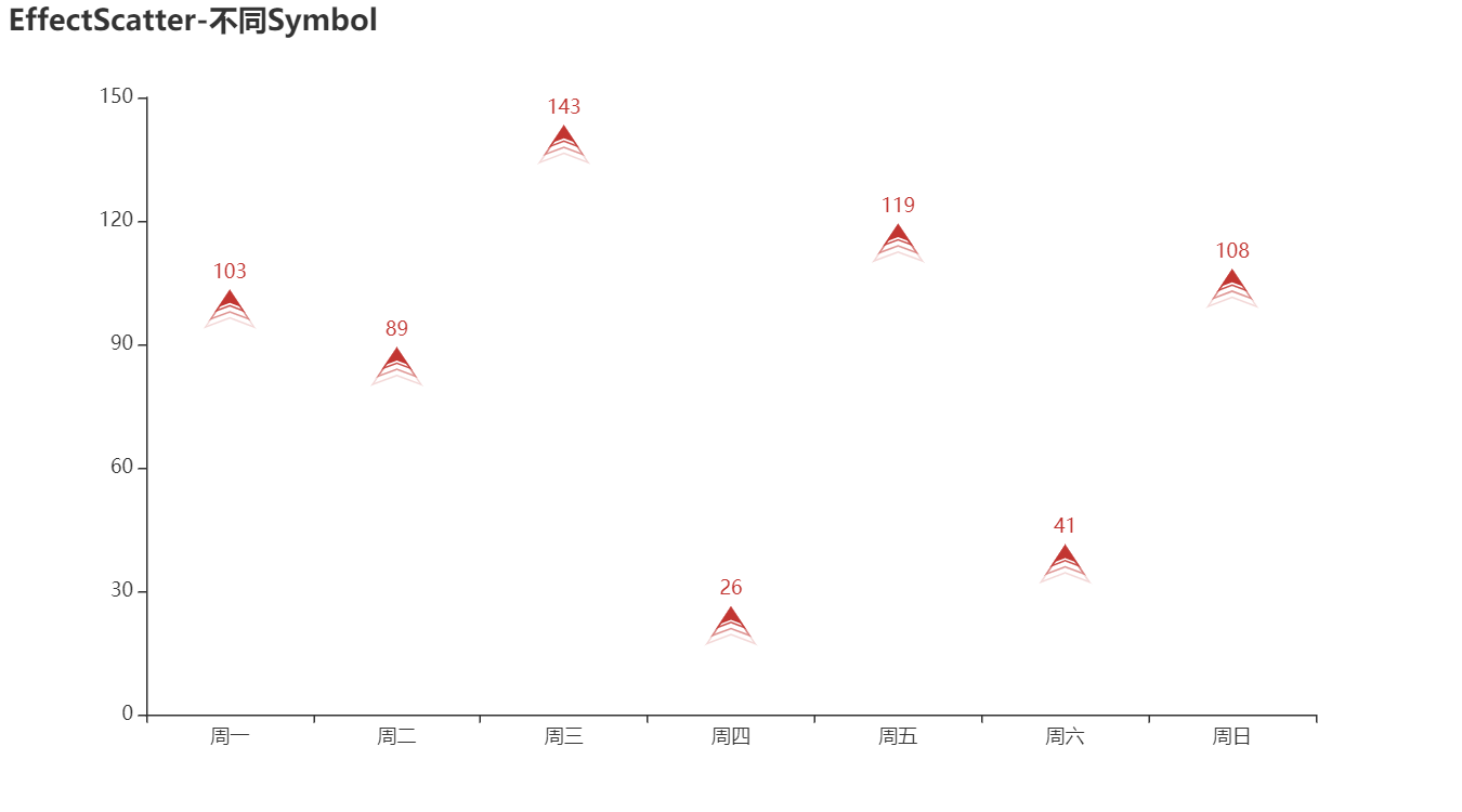
67.1 Effectscatter - Effectscatter_symbol
from pyecharts import options as opts
from pyecharts.charts import EffectScatter
from pyecharts.faker import Faker
from pyecharts.globals import SymbolType

c = (
    EffectScatter()
    .add_xaxis(Faker.choose())
    .add_yaxis("", Faker.values(), symbol=SymbolType.ARROW)
    .set_global_opts(title_opts=opts.TitleOpts(title="EffectScatter-不同Symbol"))
    .render("effectscatter_symbol.html")
)
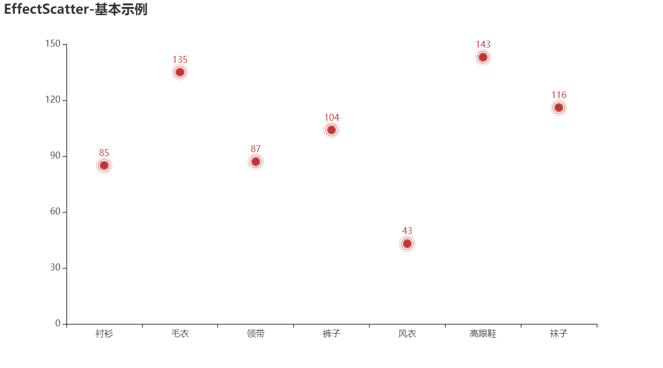
67.2 Effectscatter - Effectscatter_base
from pyecharts import options as opts
from pyecharts.charts import EffectScatter
from pyecharts.faker import Faker

c = (
    EffectScatter()
    .add_xaxis(Faker.choose())
    .add_yaxis("", Faker.values())
    .set_global_opts(title_opts=opts.TitleOpts(title="EffectScatter-基本示例"))
    .render("effectscatter_base.html")
)
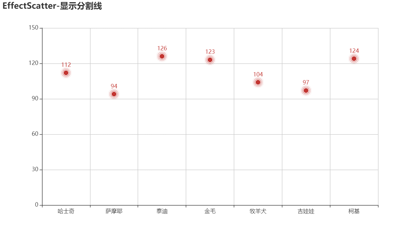
67.3 Effectscatter - Effectscatter_splitline
from pyecharts import options as opts
from pyecharts.charts import EffectScatter
from pyecharts.faker import Faker

c = (
    EffectScatter()
    .add_xaxis(Faker.choose())
    .add_yaxis("", Faker.values())
    .set_global_opts(
        title_opts=opts.TitleOpts(title="EffectScatter-显示分割线"),
        xaxis_opts=opts.AxisOpts(splitline_opts=opts.SplitLineOpts(is_show=True)),
        yaxis_opts=opts.AxisOpts(splitline_opts=opts.SplitLineOpts(is_show=True)),
    )
    .render("effectscatter_splitline.html")
)
68.HeatMap:热力图
- class pyecharts.charts.HeatMap(RectChart)
class HeatMap(
    # 初始化配置项,参考 `global_options.InitOpts`
    init_opts: opts.InitOpts = opts.InitOpts()
)
- func pyecharts.charts.HeatMap.add_yaxis
def add_yaxis(
    # 系列名称,用于 tooltip 的显示,legend 的图例筛选。
    series_name: str,

    # Y 坐标轴数据
    yaxis_data: types.Sequence[types.Union[opts.HeatMapItem, dict]],

    # 系列数据项
    value: types.Sequence[types.Union[opts.HeatMapItem, dict]],

    # 是否选中图例
    is_selected: bool = True,

    # 使用的 x 轴的 index,在单个图表实例中存在多个 x 轴的时候有用。
    xaxis_index: Optional[Numeric] = None,

    # 使用的 y 轴的 index,在单个图表实例中存在多个 y 轴的时候有用。
    yaxis_index: Optional[Numeric] = None,

    # 标签配置项,参考 `series_options.LabelOpts`
    label_opts: Union[opts.LabelOpts, dict] = opts.LabelOpts(),

    # 标记点配置项,参考 `series_options.MarkPointOpts`
    markpoint_opts: Union[opts.MarkPointOpts, dict, None] = None,

    # 标记线配置项,参考 `series_options.MarkLineOpts`
    markline_opts: Union[opts.MarkLineOpts, dict, None] = None,

    # 提示框组件配置项,参考 `series_options.TooltipOpts`
    tooltip_opts: Union[opts.TooltipOpts, dict, None] = None,

    # 图元样式配置项,参考 `series_options.ItemStyleOpts`
    itemstyle_opts: Union[opts.ItemStyleOpts, dict, None] = None,
)
- HeatMapItem:热力图数据项
class HeatMapItem(
    # 数据项名称。
    name: Optional[str] = None,

    # 数据项的值。
    value: Optional[Sequence] = None,

    # 图元样式配置项,参考 `series_options.ItemStyleOpts`
    itemstyle_opts: Union[ItemStyleOpts, dict, None] = None,

    # 提示框组件配置项,参考 `series_options.TooltipOpts`
    tooltip_opts: Union[TooltipOpts, dict, None] = None,
)
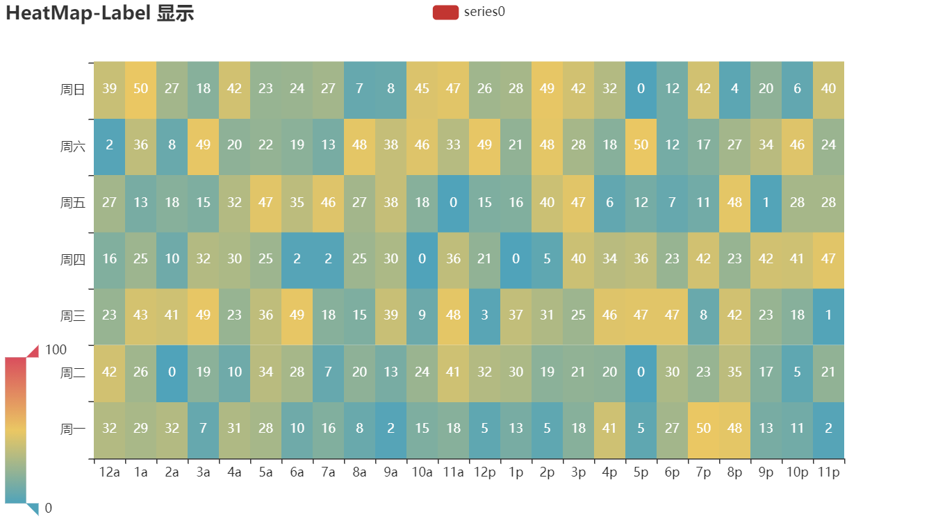
68.1 Heatmap - Heatmap_with_label_show
import random

from pyecharts import options as opts
from pyecharts.charts import HeatMap
from pyecharts.faker import Faker

value = [[i, j, random.randint(0, 50)] for i in range(24) for j in range(7)]
c = (
    HeatMap()
    .add_xaxis(Faker.clock)
    .add_yaxis(
        "series0",
        Faker.week,
        value,
        label_opts=opts.LabelOpts(is_show=True, position="inside"),
    )
    .set_global_opts(
        title_opts=opts.TitleOpts(title="HeatMap-Label 显示"),
        visualmap_opts=opts.VisualMapOpts(),
    )
    .render("heatmap_with_label_show.html")
)
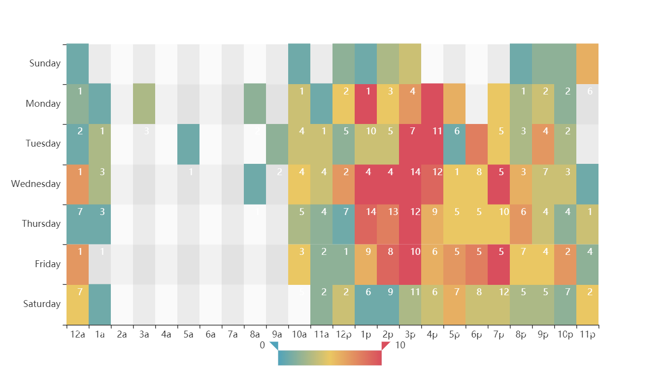
68.2 Heatmap - Heatmap_on_cartesian
import pyecharts.options as opts
from pyecharts.charts import HeatMap

"""
Gallery 使用 pyecharts 1.1.0
参考地址: https://echarts.apache.org/examples/editor.html?c=heatmap-cartesian

目前无法实现的功能:

1、官方示例中的 label 暂时无法居中,待解决
2、暂时无法对块设置 itemStyle
"""

hours = [
    "12a",
    "1a",
    "2a",
    "3a",
    "4a",
    "5a",
    "6a",
    "7a",
    "8a",
    "9a",
    "10a",
    "11a",
    "12p",
    "1p",
    "2p",
    "3p",
    "4p",
    "5p",
    "6p",
    "7p",
    "8p",
    "9p",
    "10p",
    "11p",
]
days = ["Saturday", "Friday", "Thursday", "Wednesday", "Tuesday", "Monday", "Sunday"]

data = [
    [0, 0, 5],
    [0, 1, 1],
    [0, 2, 0],
    [0, 3, 0],
    [0, 4, 0],
    [0, 5, 0],
    [0, 6, 0],
    [0, 7, 0],
    [0, 8, 0],
    [0, 9, 0],
    [0, 10, 0],
    [0, 11, 2],
    [0, 12, 4],
    [0, 13, 1],
    [0, 14, 1],
    [0, 15, 3],
    [0, 16, 4],
    [0, 17, 6],
    [0, 18, 4],
    [0, 19, 4],
    [0, 20, 3],
    [0, 21, 3],
    [0, 22, 2],
    [0, 23, 5],
    [1, 0, 7],
    [1, 1, 0],
    [1, 2, 0],
    [1, 3, 0],
    [1, 4, 0],
    [1, 5, 0],
    [1, 6, 0],
    [1, 7, 0],
    [1, 8, 0],
    [1, 9, 0],
    [1, 10, 5],
    [1, 11, 2],
    [1, 12, 2],
    [1, 13, 6],
    [1, 14, 9],
    [1, 15, 11],
    [1, 16, 6],
    [1, 17, 7],
    [1, 18, 8],
    [1, 19, 12],
    [1, 20, 5],
    [1, 21, 5],
    [1, 22, 7],
    [1, 23, 2],
    [2, 0, 1],
    [2, 1, 1],
    [2, 2, 0],
    [2, 3, 0],
    [2, 4, 0],
    [2, 5, 0],
    [2, 6, 0],
    [2, 7, 0],
    [2, 8, 0],
    [2, 9, 0],
    [2, 10, 3],
    [2, 11, 2],
    [2, 12, 1],
    [2, 13, 9],
    [2, 14, 8],
    [2, 15, 10],
    [2, 16, 6],
    [2, 17, 5],
    [2, 18, 5],
    [2, 19, 5],
    [2, 20, 7],
    [2, 21, 4],
    [2, 22, 2],
    [2, 23, 4],
    [3, 0, 7],
    [3, 1, 3],
    [3, 2, 0],
    [3, 3, 0],
    [3, 4, 0],
    [3, 5, 0],
    [3, 6, 0],
    [3, 7, 0],
    [3, 8, 1],
    [3, 9, 0],
    [3, 10, 5],
    [3, 11, 4],
    [3, 12, 7],
    [3, 13, 14],
    [3, 14, 13],
    [3, 15, 12],
    [3, 16, 9],
    [3, 17, 5],
    [3, 18, 5],
    [3, 19, 10],
    [3, 20, 6],
    [3, 21, 4],
    [3, 22, 4],
    [3, 23, 1],
    [4, 0, 1],
    [4, 1, 3],
    [4, 2, 0],
    [4, 3, 0],
    [4, 4, 0],
    [4, 5, 1],
    [4, 6, 0],
    [4, 7, 0],
    [4, 8, 0],
    [4, 9, 2],
    [4, 10, 4],
    [4, 11, 4],
    [4, 12, 2],
    [4, 13, 4],
    [4, 14, 4],
    [4, 15, 14],
    [4, 16, 12],
    [4, 17, 1],
    [4, 18, 8],
    [4, 19, 5],
    [4, 20, 3],
    [4, 21, 7],
    [4, 22, 3],
    [4, 23, 0],
    [5, 0, 2],
    [5, 1, 1],
    [5, 2, 0],
    [5, 3, 3],
    [5, 4, 0],
    [5, 5, 0],
    [5, 6, 0],
    [5, 7, 0],
    [5, 8, 2],
    [5, 9, 0],
    [5, 10, 4],
    [5, 11, 1],
    [5, 12, 5],
    [5, 13, 10],
    [5, 14, 5],
    [5, 15, 7],
    [5, 16, 11],
    [5, 17, 6],
    [5, 18, 0],
    [5, 19, 5],
    [5, 20, 3],
    [5, 21, 4],
    [5, 22, 2],
    [5, 23, 0],
    [6, 0, 1],
    [6, 1, 0],
    [6, 2, 0],
    [6, 3, 0],
    [6, 4, 0],
    [6, 5, 0],
    [6, 6, 0],
    [6, 7, 0],
    [6, 8, 0],
    [6, 9, 0],
    [6, 10, 1],
    [6, 11, 0],
    [6, 12, 2],
    [6, 13, 1],
    [6, 14, 3],
    [6, 15, 4],
    [6, 16, 0],
    [6, 17, 0],
    [6, 18, 0],
    [6, 19, 0],
    [6, 20, 1],
    [6, 21, 2],
    [6, 22, 2],
    [6, 23, 6],
]
data = [[d[1], d[0], d[2] or "-"] for d in data]


(
    HeatMap(init_opts=opts.InitOpts(width="1440px", height="720px"))
    .add_xaxis(xaxis_data=hours)
    .add_yaxis(
        series_name="Punch Card",
        yaxis_data=days,
        value=data,
        label_opts=opts.LabelOpts(
            is_show=True, color="#fff", position="bottom", horizontal_align="50%"
        ),
    )
    .set_series_opts()
    .set_global_opts(
        legend_opts=opts.LegendOpts(is_show=False),
        xaxis_opts=opts.AxisOpts(
            type_="category",
            splitarea_opts=opts.SplitAreaOpts(
                is_show=True, areastyle_opts=opts.AreaStyleOpts(opacity=1)
            ),
        ),
        yaxis_opts=opts.AxisOpts(
            type_="category",
            splitarea_opts=opts.SplitAreaOpts(
                is_show=True, areastyle_opts=opts.AreaStyleOpts(opacity=1)
            ),
        ),
        visualmap_opts=opts.VisualMapOpts(
            min_=0, max_=10, is_calculable=True, orient="horizontal", pos_left="center"
        ),
    )
    .render("heatmap_on_cartesian.html")
)
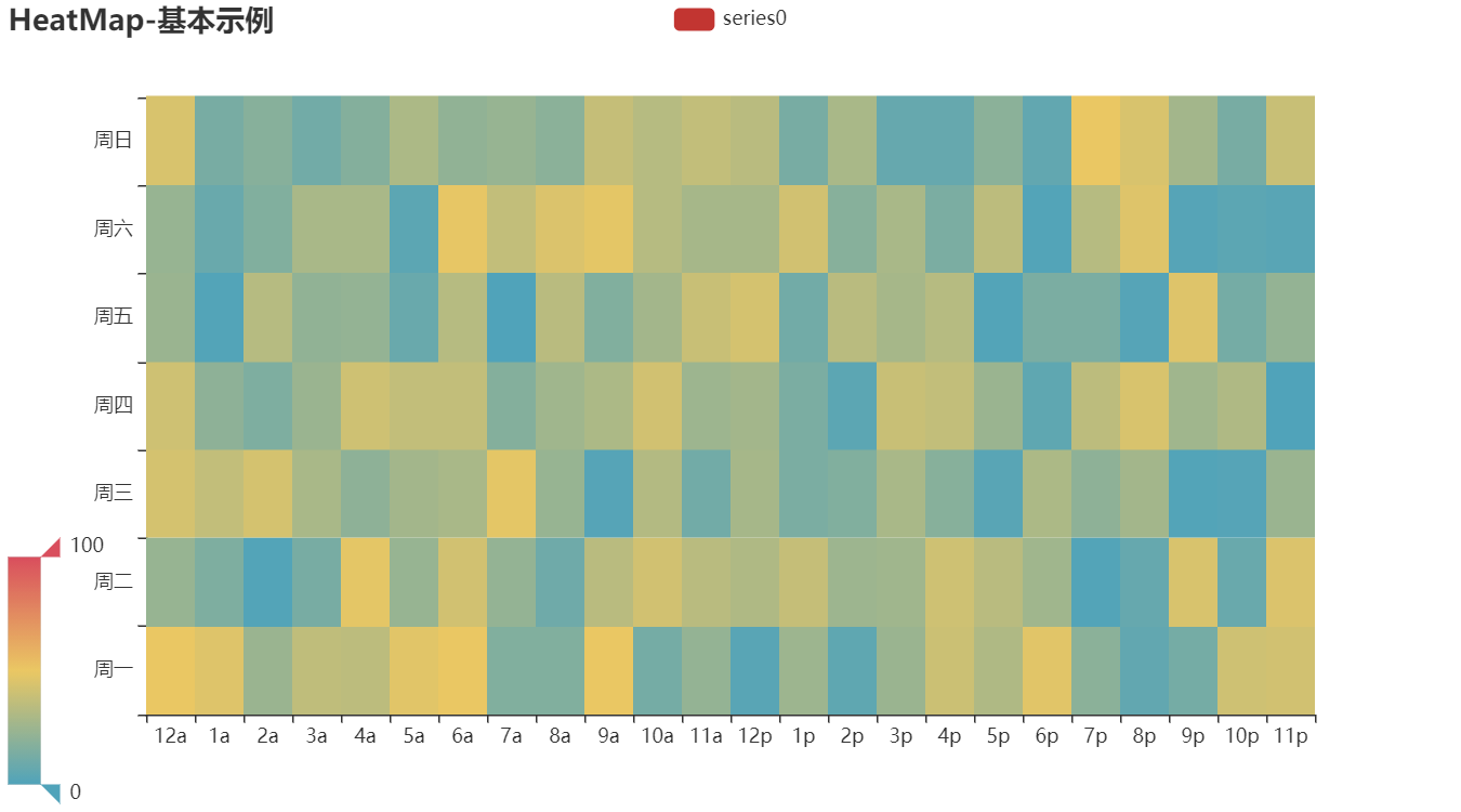
68.3 Heatmap - Heatmap_base
import random

from pyecharts import options as opts
from pyecharts.charts import HeatMap
from pyecharts.faker import Faker

value = [[i, j, random.randint(0, 50)] for i in range(24) for j in range(7)]
c = (
    HeatMap()
    .add_xaxis(Faker.clock)
    .add_yaxis("series0", Faker.week, value)
    .set_global_opts(
        title_opts=opts.TitleOpts(title="HeatMap-基本示例"),
        visualmap_opts=opts.VisualMapOpts(),
    )
    .render("heatmap_base.html")
)
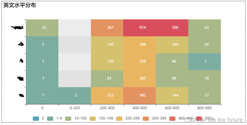
68.4 Sesaon:Heatmap实践-利用pandas和openpyxl预处理数据,一键生成pyecharts要的数据。
#################### <通过pandas来处理数据> -开始  ####################
def cate_eng(x):
    #英文分类的函数
    if x == 0:
        cate_result = "0"
    elif x > 0 and x < 200:
        cate_result = "0-200"
    elif x >= 200 and x < 400:
        cate_result = "200-400"
    elif x >= 400 and x < 600:
        cate_result = "400-600"
    elif x >= 600 and x < 800:
        cate_result = "600-800"
    elif x >= 800 and x <= 990:
        cate_result = "800-990"
    return cate_result


def cate_plant(x):
    #部门分类的函数
    if x[:3] == 'MZV':
        cate_result = "P1"
    elif x[:3] == 'MZ3':
        cate_result = "P3"
    elif x[:3] == 'MZD':
        cate_result = "P6"
    elif x[:3] == 'MZ8':
        cate_result = "P8"
    elif x[:1] == 'S':
        cate_result = "P8"
    else:
        cate_result = "others"
    return cate_result


def pandas_prepare(excel_name,sheet_name,output_excelname):
    df_row = pd.DataFrame(pd.read_excel(excel_name,sheet_name = sheet_name))
    df_row['HIGHESTSCORES'] = df_row['HIGHESTSCORES'].fillna(value=0)
    #运用apply整理数据
    df_row['HIGHESTSCORES_categary'] = df_row['HIGHESTSCORES'].apply(cate_eng)
    df_row['DEPARTMENT'] = df_row['DEPARTMENT'].apply(str)
    df_row['PlantID'] = df_row['DEPARTMENT'].apply(cate_plant)

    #导出枢纽分析表
    #table1 = pd.pivot_table(df_row, values='D', index=['A', 'B'],columns=['C'], aggfunc=np.sum)
    df2 = df_row.groupby(by=['PlantID','HIGHESTSCORES_categary']).ENGFUNC.count()


    #导出相关信息
    print(df_row.columns)

    with pd.ExcelWriter(output_excelname) as writer:
        df_row.to_excel(writer, sheet_name='English1')
        df2.to_excel(writer, sheet_name='groupby')


def Heatmap_data_prepare(output_excelname):
    #把厂别添加到第4栏
    wb = load_workbook(output_excelname)
    sheet_g = wb['groupby']
    sheet_g['D1'].value = 'PlantID2'
    sheet_g['E1'].value = 'english_index'
    sheet_g['F1'].value = 'plantid_index'
    plant_str = ''
    for i in range(2,sheet_g.max_row+1):
        if sheet_g.cell(row = i, column = 1).value:
            plant_str = sheet_g.cell(row = i, column = 1).value
            sheet_g.cell(row = i, column = 4).value = plant_str
        else:
            sheet_g.cell(row = i, column = 4).value = plant_str
    #变更分数范围的信息为数字
    for i in range(2,sheet_g.max_row+1):
        if sheet_g.cell(row = i, column = 2).value =="0":
            sheet_g.cell(row = i, column = 5).value = 0
        elif sheet_g.cell(row = i, column = 2).value =="0-200":
            sheet_g.cell(row = i, column = 5).value = 1
        elif sheet_g.cell(row = i, column = 2).value =="200-400":
            sheet_g.cell(row = i, column = 5).value = 2
        elif sheet_g.cell(row = i, column = 2).value =="400-600":
            sheet_g.cell(row = i, column = 5).value = 3
        elif sheet_g.cell(row = i, column = 2).value =="600-800":
            sheet_g.cell(row = i, column = 5).value = 4
        elif sheet_g.cell(row = i, column = 2).value =="800-990":
            sheet_g.cell(row = i, column = 5).value = 5
    #变更厂别信息的信息为数字
    for i in range(2,sheet_g.max_row+1):
        if sheet_g.cell(row = i, column = 4).value =="P1":
            sheet_g.cell(row = i, column = 6).value = 0
        elif sheet_g.cell(row = i, column = 4).value =="P3":
            sheet_g.cell(row = i, column = 6).value = 1
        elif sheet_g.cell(row = i, column = 4).value =="P6":
            sheet_g.cell(row = i, column = 6).value = 2
        elif sheet_g.cell(row = i, column = 4).value =="P8":
            sheet_g.cell(row = i, column = 6).value = 3
        elif sheet_g.cell(row = i, column = 4).value =="others":
            sheet_g.cell(row = i, column = 6).value = 4
    wb.save(output_excelname)


    #把数据打包成list传给pyecharts
    data = []
    for i in range(2,sheet_g.max_row+1):
        data_short = []
        data_short.append(sheet_g.cell(row = i, column = 5).value) #["0","0-200","200-400","400-600","600-800","800-990"]
        data_short.append(sheet_g.cell(row = i, column = 6).value) #["P1","P3","P6","P8","others"]
        data_short.append(sheet_g.cell(row = i, column = 3).value) #value
        data.append(data_short)
    print(data)
    return data


output_excelname = 'excel_to_python.xlsx'
pandas_prepare(excel_name,'English1',output_excelname)
Heatmap_data_prepare(output_excelname)
#################### <通过pandas来处理数据>-结束 ####################


def Heatmap_english():
    x_data = ["0","0-200","200-400","400-600","600-800","800-990"]
    y_data = ["P1","P3","P6","P8","others"]

    #data = [[1,1,1],[1,3,1],[1,2,1],[1,5,1],[3,0,1],[3,5,3],[3,4,1],[5,5,1],[5,5,5],]
    data = Heatmap_data_prepare(output_excelname)

    # 以下的data是关键点
    data = [[d[0], d[1], d[2] or "-"] for d in data]


    c = (
        HeatMap(init_opts=opts.InitOpts(width="800px", height="400px"))
        .add_xaxis(xaxis_data=x_data)
        .add_yaxis(
            series_name="人数",
            yaxis_data=y_data,
            value=data,
            label_opts=opts.LabelOpts(
                is_show=True, color="#fff", position="inside", horizontal_align="50%"
            ),
        )
        .set_series_opts()
        .set_global_opts(
            title_opts=opts.TitleOpts(title="英文水平分布"),
            legend_opts=opts.LegendOpts(is_show=False),
            xaxis_opts=opts.AxisOpts(
                type_="category",
                splitarea_opts=opts.SplitAreaOpts(
                    is_show=True, areastyle_opts=opts.AreaStyleOpts(opacity=1)
                ),
            ),
            yaxis_opts=opts.AxisOpts(
                type_="category",
                splitarea_opts=opts.SplitAreaOpts(
                    is_show=True, areastyle_opts=opts.AreaStyleOpts(opacity=1)
                ),
            ),
            visualmap_opts=opts.VisualMapOpts(
                is_calculable=True, orient="horizontal", pos_left="center",
                is_piecewise=True,
                pieces= [
                {"min": 500,"label": '500+'},
                {"min": 400, "max": 499, "label": '400-499'},
                {"min": 300, "max": 399, "label": '300-399'},
                {"min": 200, "max": 299, "label": '200-299'},
                {"min": 100, "max": 199, "label": '100-199'},
                {"min": 10, "max": 99, "label": '10-100'},
                {"min": 1, "max": 9, "label": '1-9'},
                {"max": 0, "label": '0'},
                ]
            ),
        )
    )
    return c
69.Kline/Candlestick:K线图
- class pyecharts.charts.Kline(RectChart)
class Kline(
    # 初始化配置项,参考 `global_options.InitOpts`
    init_opts: opts.InitOpts = opts.InitOpts()
)
- func pyecharts.charts.Kline.add_yaxis
def add_yaxis(
    # 系列名称,用于 tooltip 的显示,legend 的图例筛选。
    series_name: str,

    # 系列数据
    y_axis: types.Sequence[types.Union[opts.CandleStickItem, dict]],

    # 是否选中图例
    is_selected: bool = True,

    # 使用的 x 轴的 index,在单个图表实例中存在多个 x 轴的时候有用。
    xaxis_index: Optional[Numeric] = None,

    # 使用的 y 轴的 index,在单个图表实例中存在多个 y 轴的时候有用。
    yaxis_index: Optional[Numeric] = None,

    # 标记线配置项,参考 `series_options.MarkLineOpts`
    markline_opts: Union[opts.MarkLineOpts, dict, None] = None,

    # 标记点配置项,参考 `series_options.MarkPointOpts`
    markpoint_opts: Union[opts.MarkPointOpts, dict, None] = None,

    # 提示框组件配置项,参考 `series_options.TooltipOpts`
    tooltip_opts: Union[opts.TooltipOpts, dict, None] = None,

    # 图元样式配置项,参考 `series_options.ItemStyleOpts`
    itemstyle_opts: Union[opts.ItemStyleOpts, dict, None] = None,
)
- CandleStickItem:K 线图数据项
class CandleStickItem(
    # 数据项名称。
    name: Optional[str] = None,

    # 数据项的值。
    value: Optional[Sequence] = None,

    # 图元样式配置项,参考 `series_options.ItemStyleOpts`
    itemstyle_opts: Union[ItemStyleOpts, dict, None] = None,

    # 提示框组件配置项,参考 `series_options.TooltipOpts`
    tooltip_opts: Union[TooltipOpts, dict, None] = None,
)
?69.1 Candlestick - Professional_kline_chart
"""
复刻的 Echarts 的 demo 链接
https://gallery.echartsjs.com/editor.html?c=xByOFPcjBe
@Author: sunhailin-Leo
@Time: 2019年7月14日
"""
from typing import List, Sequence, Union
from pyecharts import options as opts
from pyecharts.commons.utils import JsCode
from pyecharts.charts import Kline, Line, Bar, Grid
# 数据
echarts_data = [
["2015-10-16", 18.4, 18.58, 18.33, 18.79, 67.00, 1, 0.04, 0.11, 0.09],
["2015-10-19", 18.56, 18.25, 18.19, 18.56, 55.00, 0, -0.00, 0.08, 0.09],
["2015-10-20", 18.3, 18.22, 18.05, 18.41, 37.00, 0, 0.01, 0.09, 0.09],
["2015-10-21", 18.18, 18.69, 18.02, 18.98, 89.00, 0, 0.03, 0.10, 0.08],
["2015-10-22", 18.42, 18.29, 18.22, 18.48, 43.00, 0, -0.06, 0.05, 0.08],
["2015-10-23", 18.26, 18.19, 18.08, 18.36, 46.00, 0, -0.10, 0.03, 0.09],
["2015-10-26", 18.33, 18.07, 17.98, 18.35, 65.00, 0, -0.15, 0.03, 0.10],
["2015-10-27", 18.08, 18.04, 17.88, 18.13, 37.00, 0, -0.19, 0.03, 0.12],
["2015-10-28", 17.96, 17.86, 17.82, 17.99, 35.00, 0, -0.24, 0.03, 0.15],
["2015-10-29", 17.85, 17.81, 17.8, 17.93, 27.00, 0, -0.24, 0.06, 0.18],
["2015-10-30", 17.79, 17.93, 17.78, 18.08, 43.00, 0, -0.22, 0.11, 0.22],
["2015-11-02", 17.78, 17.83, 17.78, 18.04, 27.00, 0, -0.20, 0.15, 0.25],
["2015-11-03", 17.84, 17.9, 17.84, 18.06, 34.00, 0, -0.12, 0.22, 0.28],
["2015-11-04", 17.97, 18.36, 17.85, 18.39, 62.00, 0, -0.00, 0.30, 0.30],
["2015-11-05", 18.3, 18.57, 18.18, 19.08, 177.00, 0, 0.07, 0.33, 0.30],
["2015-11-06", 18.53, 18.68, 18.3, 18.71, 95.00, 0, 0.12, 0.35, 0.29],
["2015-11-09", 18.75, 19.08, 18.75, 19.98, 202.00, 1, 0.16, 0.35, 0.27],
["2015-11-10", 18.85, 18.64, 18.56, 18.99, 85.00, 0, 0.09, 0.29, 0.25],
["2015-11-11", 18.64, 18.44, 18.31, 18.64, 50.00, 0, 0.06, 0.27, 0.23],
["2015-11-12", 18.55, 18.27, 18.17, 18.57, 43.00, 0, 0.05, 0.25, 0.23],
["2015-11-13", 18.13, 18.14, 18.09, 18.34, 35.00, 0, 0.05, 0.24, 0.22],
["2015-11-16", 18.01, 18.1, 17.93, 18.17, 34.00, 0, 0.07, 0.25, 0.21],
["2015-11-17", 18.2, 18.14, 18.08, 18.45, 58.00, 0, 0.11, 0.25, 0.20],
["2015-11-18", 18.23, 18.16, 18.0, 18.45, 47.00, 0, 0.13, 0.25, 0.19],
["2015-11-19", 18.08, 18.2, 18.05, 18.25, 32.00, 0, 0.15, 0.24, 0.17],
["2015-11-20", 18.15, 18.15, 18.11, 18.29, 36.00, 0, 0.13, 0.21, 0.15],
["2015-11-23", 18.16, 18.19, 18.12, 18.34, 47.00, 0, 0.11, 0.18, 0.13],
["2015-11-24", 18.23, 17.88, 17.7, 18.23, 62.00, 0, 0.03, 0.13, 0.11],
["2015-11-25", 17.85, 17.73, 17.56, 17.85, 66.00, 0, -0.03, 0.09, 0.11],
["2015-11-26", 17.79, 17.53, 17.5, 17.92, 63.00, 0, -0.10, 0.06, 0.11],
["2015-11-27", 17.51, 17.04, 16.9, 17.51, 67.00, 0, -0.16, 0.05, 0.13],
["2015-11-30", 17.07, 17.2, 16.98, 17.32, 55.00, 0, -0.12, 0.09, 0.15],
["2015-12-01", 17.28, 17.11, 16.91, 17.28, 39.00, 0, -0.09, 0.12, 0.16],
["2015-12-02", 17.13, 17.91, 17.05, 17.99, 102.00, 0, -0.01, 0.17, 0.18],
["2015-12-03", 17.8, 17.78, 17.61, 17.98, 71.00, 0, -0.09, 0.14, 0.18],
["2015-12-04", 17.6, 17.25, 17.13, 17.69, 51.00, 0, -0.18, 0.10, 0.19],
["2015-12-07", 17.2, 17.39, 17.15, 17.45, 43.00, 0, -0.19, 0.12, 0.22],
["2015-12-08", 17.3, 17.42, 17.18, 17.62, 45.00, 0, -0.23, 0.13, 0.24],
["2015-12-09", 17.33, 17.39, 17.32, 17.59, 44.00, 0, -0.29, 0.13, 0.28],
["2015-12-10", 17.39, 17.26, 17.21, 17.65, 44.00, 0, -0.37, 0.13, 0.32],
["2015-12-11", 17.23, 16.92, 16.66, 17.26, 114.00, 1, -0.44, 0.15, 0.37],
["2015-12-14", 16.75, 17.06, 16.5, 17.09, 94.00, 0, -0.44, 0.21, 0.44],
["2015-12-15", 17.03, 17.03, 16.9, 17.06, 46.00, 0, -0.44, 0.28, 0.50],
["2015-12-16", 17.08, 16.96, 16.87, 17.09, 30.00, 0, -0.40, 0.36, 0.56],
["2015-12-17", 17.0, 17.1, 16.95, 17.12, 50.00, 0, -0.30, 0.47, 0.62],
["2015-12-18", 17.09, 17.52, 17.04, 18.06, 156.00, 0, -0.14, 0.59, 0.66],
["2015-12-21", 17.43, 18.23, 17.35, 18.45, 152.00, 1, 0.02, 0.69, 0.68],
["2015-12-22", 18.14, 18.27, 18.06, 18.32, 94.00, 0, 0.08, 0.72, 0.68],
["2015-12-23", 18.28, 18.19, 18.17, 18.71, 108.00, 0, 0.13, 0.73, 0.67],
["2015-12-24", 18.18, 18.14, 18.01, 18.31, 37.00, 0, 0.19, 0.74, 0.65],
["2015-12-25", 18.22, 18.33, 18.2, 18.36, 48.00, 0, 0.26, 0.75, 0.62],
["2015-12-28", 18.35, 17.84, 17.8, 18.39, 48.00, 0, 0.27, 0.72, 0.59],
["2015-12-29", 17.83, 17.94, 17.71, 17.97, 36.00, 0, 0.36, 0.73, 0.55],
["2015-12-30", 17.9, 18.26, 17.55, 18.3, 71.00, 1, 0.43, 0.71, 0.50],
["2015-12-31", 18.12, 17.99, 17.91, 18.33, 72.00, 0, 0.40, 0.63, 0.43],
["2016-01-04", 17.91, 17.28, 17.16, 17.95, 37.00, 1, 0.34, 0.55, 0.38],
["2016-01-05", 17.17, 17.23, 17.0, 17.55, 51.00, 0, 0.37, 0.51, 0.33],
["2016-01-06", 17.2, 17.31, 17.06, 17.33, 31.00, 0, 0.37, 0.46, 0.28],
["2016-01-07", 17.15, 16.67, 16.51, 17.15, 19.00, 0, 0.30, 0.37, 0.22],
["2016-01-08", 16.8, 16.81, 16.61, 17.06, 60.00, 0, 0.29, 0.32, 0.18],
["2016-01-11", 16.68, 16.04, 16.0, 16.68, 65.00, 0, 0.20, 0.24, 0.14],
["2016-01-12", 16.03, 15.98, 15.88, 16.25, 46.00, 0, 0.20, 0.21, 0.11],
["2016-01-13", 16.21, 15.87, 15.78, 16.21, 57.00, 0, 0.20, 0.18, 0.08],
["2016-01-14", 15.55, 15.89, 15.52, 15.96, 42.00, 0, 0.20, 0.16, 0.05],
["2016-01-15", 15.87, 15.48, 15.45, 15.92, 34.00, 1, 0.17, 0.11, 0.02],
["2016-01-18", 15.39, 15.42, 15.36, 15.7, 26.00, 0, 0.21, 0.10, -0.00],
["2016-01-19", 15.58, 15.71, 15.35, 15.77, 38.00, 0, 0.25, 0.09, -0.03],
["2016-01-20", 15.56, 15.52, 15.24, 15.68, 38.00, 0, 0.23, 0.05, -0.07],
["2016-01-21", 15.41, 15.3, 15.28, 15.68, 35.00, 0, 0.21, 0.00, -0.10],
["2016-01-22", 15.48, 15.28, 15.13, 15.49, 30.00, 0, 0.21, -0.02, -0.13],
["2016-01-25", 15.29, 15.48, 15.2, 15.49, 21.00, 0, 0.20, -0.06, -0.16],
["2016-01-26", 15.33, 14.86, 14.78, 15.39, 30.00, 0, 0.12, -0.13, -0.19],
["2016-01-27", 14.96, 15.0, 14.84, 15.22, 51.00, 0, 0.13, -0.14, -0.20],
["2016-01-28", 14.96, 14.72, 14.62, 15.06, 25.00, 0, 0.10, -0.17, -0.22],
["2016-01-29", 14.75, 14.99, 14.62, 15.08, 36.00, 0, 0.13, -0.17, -0.24],
["2016-02-01", 14.98, 14.72, 14.48, 15.18, 27.00, 0, 0.10, -0.21, -0.26],
["2016-02-02", 14.65, 14.85, 14.65, 14.95, 18.00, 0, 0.11, -0.21, -0.27],
["2016-02-03", 14.72, 14.67, 14.55, 14.8, 23.00, 0, 0.10, -0.24, -0.29],
["2016-02-04", 14.79, 14.88, 14.69, 14.93, 22.00, 0, 0.13, -0.24, -0.30],
["2016-02-05", 14.9, 14.86, 14.78, 14.93, 16.00, 0, 0.12, -0.26, -0.32],
["2016-02-15", 14.5, 14.66, 14.47, 14.82, 19.00, 0, 0.11, -0.28, -0.34],
["2016-02-16", 14.77, 14.94, 14.72, 15.05, 26.00, 0, 0.14, -0.28, -0.35],
["2016-02-17", 14.95, 15.03, 14.88, 15.07, 38.00, 0, 0.12, -0.31, -0.37],
["2016-02-18", 14.95, 14.9, 14.87, 15.06, 28.00, 0, 0.07, -0.35, -0.39],
["2016-02-19", 14.9, 14.75, 14.68, 14.94, 22.00, 0, 0.03, -0.38, -0.40],
["2016-02-22", 14.88, 15.01, 14.79, 15.11, 38.00, 1, 0.01, -0.40, -0.40],
["2016-02-23", 15.01, 14.83, 14.72, 15.01, 24.00, 0, -0.09, -0.45, -0.40],
["2016-02-24", 14.75, 14.81, 14.67, 14.87, 21.00, 0, -0.17, -0.48, -0.39],
["2016-02-25", 14.81, 14.25, 14.21, 14.81, 51.00, 1, -0.27, -0.50, -0.37],
["2016-02-26", 14.35, 14.45, 14.28, 14.57, 28.00, 0, -0.26, -0.46, -0.33],
["2016-02-29", 14.43, 14.56, 14.04, 14.6, 48.00, 0, -0.25, -0.41, -0.29],
["2016-03-01", 14.56, 14.65, 14.36, 14.78, 32.00, 0, -0.21, -0.36, -0.25],
["2016-03-02", 14.79, 14.96, 14.72, 14.97, 60.00, 0, -0.13, -0.29, -0.22],
["2016-03-03", 14.95, 15.15, 14.91, 15.19, 53.00, 1, -0.05, -0.23, -0.21],
["2016-03-04", 15.14, 15.97, 15.02, 16.02, 164.00, 1, 0.06, -0.17, -0.20],
["2016-03-07", 15.9, 15.78, 15.65, 16.0, 41.00, 0, 0.04, -0.19, -0.21],
["2016-03-08", 15.78, 15.96, 15.21, 15.99, 45.00, 0, 0.05, -0.19, -0.21],
["2016-03-09", 15.73, 16.05, 15.41, 16.08, 74.00, 0, 0.03, -0.20, -0.22],
["2016-03-10", 15.82, 15.66, 15.65, 15.98, 19.00, 0, -0.02, -0.23, -0.22],
["2016-03-11", 15.59, 15.76, 15.42, 15.78, 32.00, 0, 0.01, -0.22, -0.22],
["2016-03-14", 15.78, 15.72, 15.65, 16.04, 31.00, 0, 0.03, -0.20, -0.22],
["2016-03-15", 15.81, 15.86, 15.6, 15.99, 35.00, 0, 0.10, -0.18, -0.23],
["2016-03-16", 15.88, 16.42, 15.79, 16.45, 123.00, 0, 0.17, -0.16, -0.24],
["2016-03-17", 16.39, 16.23, 16.11, 16.4, 46.00, 0, 0.14, -0.20, -0.26],
["2016-03-18", 16.39, 16.17, 16.04, 16.4, 59.00, 0, 0.13, -0.22, -0.28],
["2016-03-21", 16.21, 16.22, 16.11, 16.44, 50.00, 0, 0.12, -0.24, -0.30],
["2016-03-22", 16.27, 16.19, 16.16, 16.42, 33.00, 0, 0.10, -0.27, -0.32],
["2016-03-23", 16.26, 16.18, 16.18, 16.29, 19.00, 0, 0.08, -0.30, -0.33],
["2016-03-24", 16.18, 16.11, 16.01, 16.23, 23.00, 0, 0.04, -0.33, -0.35],
["2016-03-25", 16.12, 16.13, 16.1, 16.2, 15.00, 0, 0.00, -0.35, -0.35],
["2016-03-28", 16.15, 15.85, 15.81, 16.2, 22.00, 0, -0.06, -0.38, -0.35],
["2016-03-29", 15.9, 15.79, 15.76, 16.05, 19.00, 0, -0.06, -0.37, -0.34],
["2016-03-30", 15.79, 16.24, 15.78, 16.3, 29.00, 0, -0.03, -0.35, -0.33],
["2016-03-31", 16.3, 16.09, 16.02, 16.35, 25.00, 0, -0.07, -0.37, -0.33],
["2016-04-01", 16.18, 16.27, 15.98, 16.3, 38.00, 0, -0.08, -0.36, -0.32],
["2016-04-05", 16.13, 16.34, 16.07, 16.37, 39.00, 0, -0.13, -0.37, -0.31],
["2016-04-06", 16.21, 16.26, 16.19, 16.35, 30.00, 0, -0.20, -0.39, -0.29],
["2016-04-07", 16.32, 16.1, 16.05, 16.35, 29.00, 1, -0.26, -0.39, -0.26],
["2016-04-08", 16.0, 16.16, 15.98, 16.21, 22.00, 0, -0.28, -0.37, -0.23],
["2016-04-11", 16.16, 16.31, 16.15, 16.57, 31.00, 0, -0.30, -0.33, -0.19],
["2016-04-12", 16.41, 16.29, 16.12, 16.41, 17.00, 0, -0.31, -0.30, -0.14],
["2016-04-13", 16.39, 16.48, 16.0, 16.68, 40.00, 0, -0.30, -0.25, -0.10],
["2016-04-14", 16.5, 16.46, 16.37, 16.68, 22.00, 0, -0.27, -0.19, -0.06],
["2016-04-15", 16.56, 16.93, 16.46, 17.04, 58.00, 0, -0.20, -0.12, -0.02],
["2016-04-18", 16.76, 17.06, 16.72, 17.27, 50.00, 0, -0.16, -0.07, 0.01],
["2016-04-19", 17.21, 17.11, 17.02, 17.23, 30.00, 0, -0.12, -0.02, 0.03],
["2016-04-20", 17.11, 17.33, 16.8, 17.36, 78.00, 0, -0.04, 0.03, 0.05],
["2016-04-21", 17.27, 17.69, 17.17, 17.93, 79.00, 0, 0.05, 0.08, 0.06],
["2016-04-22", 17.6, 17.87, 17.56, 18.02, 55.00, 0, 0.09, 0.10, 0.05],
["2016-04-25", 17.75, 17.9, 17.41, 17.96, 39.00, 1, 0.11, 0.09, 0.04],
["2016-04-26", 17.81, 17.91, 17.6, 17.95, 39.00, 0, 0.12, 0.08, 0.02],
["2016-04-27", 17.9, 17.88, 17.81, 17.95, 25.00, 0, 0.12, 0.06, 0.00],
["2016-04-28", 17.93, 17.88, 17.67, 17.93, 28.00, 0, 0.11, 0.04, -0.01],
["2016-04-29", 17.87, 17.75, 17.73, 17.92, 19.00, 0, 0.08, 0.01, -0.03],
["2016-05-03", 17.79, 17.7, 17.56, 17.85, 35.00, 0, 0.05, -0.01, -0.04],
["2016-05-04", 17.7, 17.65, 17.59, 17.71, 24.00, 0, 0.02, -0.04, -0.05],
["2016-05-05", 17.65, 17.62, 17.46, 17.7, 20.00, 0, -0.03, -0.06, -0.05],
["2016-05-06", 17.62, 17.32, 17.3, 17.65, 29.00, 0, -0.10, -0.09, -0.05],
["2016-05-09", 17.33, 17.3, 17.21, 17.45, 23.00, 0, -0.13, -0.10, -0.03],
["2016-05-10", 17.11, 17.04, 16.98, 17.41, 28.00, 0, -0.15, -0.09, -0.01],
["2016-05-11", 17.06, 17.15, 17.06, 17.32, 20.00, 0, -0.12, -0.05, 0.01],
["2016-05-12", 17.02, 17.46, 17.02, 17.58, 26.00, 0, -0.07, -0.01, 0.03],
["2016-05-13", 17.41, 17.57, 17.34, 17.62, 23.00, 0, -0.06, 0.01, 0.03],
["2016-05-16", 17.55, 17.5, 17.48, 17.64, 37.00, 0, -0.06, 0.01, 0.04],
["2016-05-17", 17.49, 17.48, 17.39, 17.53, 13.00, 0, -0.03, 0.03, 0.05],
["2016-05-18", 17.41, 17.82, 17.39, 17.87, 46.00, 0, 0.01, 0.06, 0.06],
["2016-05-19", 17.74, 17.81, 17.67, 17.86, 17.00, 0, -0.01, 0.05, 0.05],
["2016-05-20", 17.76, 17.88, 17.7, 17.93, 14.00, 0, -0.03, 0.04, 0.06],
["2016-05-23", 17.88, 17.52, 17.48, 17.97, 16.00, 0, -0.09, 0.02, 0.06],
["2016-05-24", 17.51, 17.33, 17.32, 17.51, 8.00, 0, -0.09, 0.03, 0.07],
["2016-05-25", 17.59, 17.55, 17.44, 17.59, 10.00, 0, -0.03, 0.07, 0.08],
["2016-05-26", 17.5, 17.69, 17.5, 17.8, 12.00, 0, 0.00, 0.09, 0.09],
["2016-05-27", 17.77, 17.66, 17.62, 17.77, 7.00, 0, 0.03, 0.10, 0.09],
["2016-05-30", 17.75, 17.84, 17.62, 17.87, 20.00, 0, 0.08, 0.12, 0.08],
["2016-05-31", 17.88, 18.0, 17.81, 18.03, 41.00, 0, 0.10, 0.12, 0.07],
["2016-06-01", 18.09, 17.83, 17.73, 18.09, 22.00, 0, 0.08, 0.10, 0.06],
["2016-06-02", 17.82, 17.73, 17.66, 17.88, 10.00, 0, 0.07, 0.08, 0.05],
["2016-06-03", 17.8, 17.78, 17.71, 17.83, 9.00, 0, 0.08, 0.08, 0.04],
["2016-06-06", 17.73, 17.64, 17.56, 17.83, 12.00, 0, 0.07, 0.06, 0.03],
["2016-06-07", 17.76, 17.8, 17.59, 17.87, 11.00, 0, 0.08, 0.06, 0.02],
["2016-06-08", 17.75, 17.77, 17.65, 17.84, 9.00, 0, 0.04, 0.03, 0.01],
["2016-06-13", 17.58, 17.32, 17.29, 17.79, 16.00, 0, -0.02, -0.01, 0.00],
["2016-06-14", 17.33, 17.38, 17.29, 17.5, 10.00, 0, -0.01, 0.00, 0.00],
["2016-06-15", 17.25, 17.39, 17.25, 17.46, 18.00, 0, 0.00, 0.01, 0.00],
["2016-06-16", 17.26, 17.4, 17.26, 17.46, 22.00, 0, 0.01, 0.01, 0.00],
["2016-06-17", 17.38, 17.5, 17.37, 17.67, 13.00, 0, 0.03, 0.02, 0.00],
["2016-06-20", 17.62, 17.51, 17.42, 17.63, 15.00, 0, 0.03, 0.01, -0.00],
["2016-06-21", 17.53, 17.54, 17.5, 17.7, 11.00, 0, 0.02, 0.00, -0.01],
["2016-06-22", 17.5, 17.5, 17.46, 17.6, 10.00, 0, -0.01, -0.01, -0.01],
["2016-06-23", 17.52, 17.26, 17.24, 17.53, 16.00, 0, -0.04, -0.03, -0.01],
["2016-06-24", 17.26, 17.25, 17.18, 17.38, 60.00, 0, -0.03, -0.02, -0.00],
["2016-06-27", 17.25, 17.28, 17.18, 17.33, 19.00, 0, -0.01, -0.00, 0.00],
["2016-06-28", 17.25, 17.29, 17.21, 17.32, 13.00, 0, 0.02, 0.01, 0.00],
["2016-06-29", 17.31, 17.45, 17.27, 17.49, 21.00, 0, 0.07, 0.04, 0.00],
["2016-06-30", 17.47, 17.5, 17.39, 17.55, 17.00, 0, 0.11, 0.04, -0.01],
["2016-07-01", 17.5, 17.63, 17.49, 17.66, 10.00, 0, 0.14, 0.05, -0.03],
["2016-07-04", 17.63, 17.72, 17.63, 17.92, 17.00, 0, 0.16, 0.03, -0.05],
["2016-07-05", 17.79, 17.56, 17.45, 17.79, 18.00, 0, 0.14, 0.00, -0.07],
["2016-07-06", 17.53, 17.42, 17.31, 17.54, 20.00, 0, 0.14, -0.02, -0.09],
["2016-07-07", 17.41, 17.51, 17.35, 17.52, 15.00, 0, 0.16, -0.03, -0.11],
["2016-07-08", 17.5, 17.39, 17.35, 17.51, 15.00, 0, 0.16, -0.05, -0.13],
["2016-07-11", 17.49, 17.48, 17.4, 17.55, 16.00, 0, 0.17, -0.07, -0.15],
["2016-07-12", 17.48, 17.71, 17.46, 17.75, 25.00, 0, 0.16, -0.10, -0.18],
["2016-07-13", 17.13, 17.05, 17.02, 17.39, 28.00, 0, 0.07, -0.17, -0.20],
["2016-07-14", 17.07, 17.09, 17.0, 17.16, 12.00, 0, 0.08, -0.17, -0.21],
["2016-07-15", 17.08, 17.14, 17.08, 17.17, 11.00, 0, 0.09, -0.18, -0.22],
["2016-07-18", 17.15, 17.26, 17.13, 17.49, 24.00, 0, 0.10, -0.19, -0.23],
["2016-07-19", 17.26, 17.12, 17.09, 17.33, 13.00, 0, 0.07, -0.21, -0.25],
["2016-07-20", 17.1, 17.07, 17.02, 17.14, 11.00, 0, 0.06, -0.23, -0.26],
["2016-07-21", 17.07, 17.24, 17.07, 17.27, 14.00, 0, 0.07, -0.23, -0.27],
["2016-07-22", 17.25, 17.08, 17.03, 17.25, 10.00, 0, 0.04, -0.26, -0.28],
["2016-07-25", 17.09, 17.12, 17.01, 17.18, 8.00, 0, 0.04, -0.26, -0.28],
["2016-07-26", 17.05, 17.17, 17.05, 17.2, 11.00, 0, 0.04, -0.27, -0.29],
["2016-07-27", 17.2, 17.37, 16.89, 17.38, 32.00, 0, 0.02, -0.28, -0.29],
["2016-07-28", 17.19, 17.14, 17.09, 17.29, 19.00, 0, -0.04, -0.32, -0.30],
["2016-07-29", 17.15, 17.16, 17.04, 17.23, 12.00, 0, -0.08, -0.33, -0.29],
["2016-08-01", 17.15, 17.18, 17.1, 17.24, 19.00, 0, -0.13, -0.34, -0.28],
["2016-08-02", 17.21, 17.15, 17.12, 17.25, 9.00, 0, -0.19, -0.36, -0.26],
["2016-08-03", 17.08, 17.07, 17.01, 17.16, 9.00, 0, -0.25, -0.36, -0.24],
["2016-08-04", 17.11, 17.06, 16.98, 17.12, 11.00, 1, -0.29, -0.35, -0.20],
["2016-08-05", 17.06, 17.1, 17.05, 17.15, 16.00, 0, -0.33, -0.32, -0.16],
["2016-08-08", 17.14, 17.13, 17.07, 17.15, 13.00, 0, -0.35, -0.29, -0.11],
["2016-08-09", 17.13, 17.17, 17.1, 17.2, 25.00, 0, -0.35, -0.24, -0.06],
["2016-08-10", 17.17, 17.28, 17.15, 17.29, 18.00, 0, -0.31, -0.17, -0.01],
["2016-08-11", 17.3, 17.45, 17.26, 17.87, 31.00, 0, -0.24, -0.09, 0.03],
["2016-08-12", 17.51, 17.99, 17.47, 18.0, 44.00, 0, -0.14, -0.00, 0.07],
["2016-08-15", 18.1, 18.42, 18.02, 18.99, 81.00, 0, -0.09, 0.04, 0.09],
["2016-08-16", 18.64, 18.31, 18.12, 18.87, 60.00, 0, -0.10, 0.05, 0.10],
["2016-08-17", 18.43, 18.4, 18.31, 18.68, 21.00, 0, -0.08, 0.08, 0.11],
["2016-08-18", 18.33, 18.23, 18.13, 18.65, 32.00, 0, -0.07, 0.09, 0.13],
["2016-08-19", 18.34, 18.62, 18.31, 18.75, 39.00, 0, 0.00, 0.14, 0.14],
["2016-08-22", 18.62, 18.69, 18.51, 18.8, 20.00, 0, 0.01, 0.14, 0.13],
["2016-08-23", 18.61, 18.66, 18.52, 19.0, 28.00, 0, 0.01, 0.14, 0.13],
["2016-08-24", 18.66, 18.62, 18.43, 18.7, 19.00, 0, 0.00, 0.13, 0.13],
["2016-08-25", 18.57, 18.51, 18.19, 18.64, 19.00, 0, -0.00, 0.13, 0.13],
["2016-08-26", 18.49, 18.55, 18.44, 18.6, 16.00, 0, 0.01, 0.13, 0.13],
["2016-08-29", 18.46, 18.27, 18.03, 18.48, 20.00, 0, 0.01, 0.13, 0.13],
["2016-08-30", 18.24, 18.44, 18.23, 18.52, 19.00, 0, 0.07, 0.17, 0.13],
["2016-08-31", 18.36, 18.63, 18.36, 18.76, 15.00, 0, 0.13, 0.18, 0.12],
["2016-09-01", 18.6, 18.62, 18.55, 18.78, 15.00, 0, 0.16, 0.18, 0.10],
["2016-09-02", 18.52, 18.68, 18.48, 18.72, 17.00, 0, 0.19, 0.17, 0.08],
["2016-09-05", 18.68, 18.75, 18.57, 18.82, 19.00, 0, 0.20, 0.15, 0.05],
["2016-09-06", 18.75, 18.51, 18.43, 18.78, 17.00, 0, 0.18, 0.11, 0.02],
["2016-09-07", 18.51, 18.56, 18.4, 18.62, 17.00, 0, 0.17, 0.08, -0.00],
["2016-09-08", 18.58, 18.53, 18.48, 18.63, 8.00, 0, 0.13, 0.04, -0.03],
["2016-09-09", 18.52, 18.33, 18.31, 18.57, 8.00, 0, 0.06, -0.02, -0.05],
["2016-09-12", 18.16, 17.9, 17.81, 18.18, 28.00, 0, -0.02, -0.07, -0.06],
["2016-09-13", 17.91, 17.91, 17.9, 18.08, 13.00, 0, -0.05, -0.08, -0.05],
["2016-09-14", 17.99, 17.54, 17.48, 17.99, 22.00, 0, -0.09, -0.09, -0.05],
["2016-09-19", 17.55, 17.81, 17.55, 17.88, 16.00, 0, -0.06, -0.06, -0.03],
["2016-09-20", 17.8, 17.74, 17.67, 17.85, 10.00, 0, -0.06, -0.05, -0.02],
["2016-09-21", 17.75, 17.88, 17.75, 17.95, 7.00, 0, -0.03, -0.03, -0.02],
["2016-09-22", 17.99, 17.97, 17.88, 18.17, 12.00, 0, -0.02, -0.02, -0.01],
["2016-09-23", 17.99, 17.98, 17.93, 18.09, 13.00, 0, -0.01, -0.01, -0.01],
["2016-09-26", 17.91, 18.0, 17.85, 18.09, 14.00, 0, -0.00, -0.01, -0.01],
["2016-09-27", 17.97, 18.07, 17.94, 18.1, 10.00, 0, 0.00, -0.01, -0.01],
["2016-09-28", 18.06, 17.89, 17.83, 18.06, 10.00, 0, -0.00, -0.01, -0.01],
["2016-09-29", 17.96, 18.0, 17.92, 18.07, 10.00, 0, 0.03, 0.01, -0.01],
["2016-09-30", 17.96, 18.0, 17.95, 18.1, 8.00, 0, 0.06, 0.02, -0.01],
["2016-10-10", 18.03, 18.3, 18.03, 18.38, 19.00, 0, 0.11, 0.04, -0.02],
["2016-10-11", 18.33, 18.33, 18.26, 18.49, 12.00, 0, 0.10, 0.02, -0.04],
["2016-10-12", 18.28, 18.15, 18.1, 18.31, 10.00, 0, 0.07, -0.02, -0.05],
["2016-10-13", 18.15, 18.09, 18.05, 18.21, 10.00, 0, 0.06, -0.03, -0.06],
["2016-10-14", 18.1, 18.1, 18.0, 18.15, 12.00, 0, 0.04, -0.05, -0.07],
["2016-10-17", 18.07, 17.86, 17.83, 18.1, 12.00, 0, 0.01, -0.07, -0.08],
["2016-10-18", 17.86, 17.93, 17.84, 17.99, 14.00, 0, 0.03, -0.07, -0.08],
["2016-10-19", 17.93, 17.88, 17.83, 18.05, 11.00, 0, 0.03, -0.07, -0.08],
["2016-10-20", 17.9, 17.89, 17.83, 17.98, 12.00, 0, 0.05, -0.06, -0.09],
["2016-10-21", 17.91, 17.91, 17.82, 17.93, 12.00, 0, 0.07, -0.06, -0.09],
["2016-10-24", 17.93, 18.31, 17.86, 18.42, 29.00, 0, 0.11, -0.05, -0.10],
["2016-10-25", 18.31, 18.13, 18.09, 18.46, 19.00, 0, 0.06, -0.09, -0.12],
["2016-10-26", 18.12, 17.97, 17.95, 18.15, 14.00, 0, 0.02, -0.12, -0.13],
["2016-10-27", 18.06, 17.81, 17.77, 18.06, 21.00, 0, -0.01, -0.13, -0.13],
["2016-10-28", 17.8, 17.9, 17.8, 18.05, 20.00, 0, -0.01, -0.13, -0.13],
["2016-10-31", 17.87, 17.86, 17.72, 17.96, 12.00, 0, -0.02, -0.14, -0.13],
["2016-11-01", 17.87, 17.98, 17.79, 17.99, 18.00, 0, -0.03, -0.14, -0.12],
["2016-11-02", 17.86, 17.84, 17.76, 17.94, 30.00, 0, -0.06, -0.15, -0.12],
["2016-11-03", 17.83, 17.93, 17.79, 17.97, 27.00, 0, -0.07, -0.14, -0.11],
["2016-11-04", 17.9, 17.91, 17.87, 18.0, 26.00, 0, -0.09, -0.15, -0.10],
["2016-11-07", 17.91, 17.89, 17.85, 17.93, 20.00, 0, -0.11, -0.14, -0.09],
["2016-11-08", 17.92, 17.99, 17.89, 18.06, 26.00, 0, -0.12, -0.13, -0.07],
["2016-11-09", 18.0, 17.89, 17.77, 18.08, 34.00, 0, -0.15, -0.13, -0.06],
["2016-11-10", 17.95, 18.0, 17.94, 18.11, 27.00, 0, -0.15, -0.11, -0.03],
["2016-11-11", 17.95, 18.02, 17.93, 18.08, 27.00, 0, -0.17, -0.10, -0.01],
["2016-11-14", 18.0, 18.04, 17.95, 18.25, 35.00, 0, -0.18, -0.08, 0.01],
["2016-11-15", 18.1, 18.18, 18.03, 18.24, 25.00, 0, -0.18, -0.06, 0.04],
["2016-11-16", 18.23, 18.12, 18.05, 18.29, 23.00, 0, -0.21, -0.04, 0.06],
["2016-11-17", 18.11, 18.12, 18.01, 18.14, 27.00, 0, -0.21, -0.01, 0.09],
["2016-11-18", 18.12, 18.1, 18.03, 18.16, 18.00, 0, -0.19, 0.03, 0.12],
["2016-11-21", 18.08, 18.34, 18.08, 18.68, 41.00, 0, -0.13, 0.08, 0.15],
["2016-11-22", 18.37, 18.37, 18.28, 18.49, 52.00, 0, -0.09, 0.12, 0.17],
["2016-11-23", 18.4, 18.84, 18.37, 18.9, 66.00, 0, -0.02, 0.17, 0.18],
["2016-11-24", 18.77, 18.74, 18.61, 18.97, 26.00, 0, -0.02, 0.17, 0.18],
["2016-11-25", 18.8, 18.99, 18.66, 19.02, 40.00, 0, -0.01, 0.18, 0.19],
["2016-11-28", 19.1, 18.65, 18.52, 19.2, 85.00, 0, -0.06, 0.16, 0.19],
["2016-11-29", 18.65, 18.75, 18.51, 18.76, 49.00, 0, -0.06, 0.17, 0.20],
["2016-11-30", 18.76, 18.55, 18.47, 18.82, 39.00, 0, -0.08, 0.17, 0.21],
["2016-12-01", 18.55, 18.49, 18.41, 18.64, 53.00, 0, -0.06, 0.19, 0.22],
["2016-12-02", 18.53, 18.49, 18.24, 18.54, 48.00, 0, -0.02, 0.21, 0.23],
["2016-12-05", 18.39, 18.66, 18.34, 18.67, 50.00, 0, 0.03, 0.25, 0.23],
["2016-12-06", 18.66, 18.6, 18.57, 18.78, 31.00, 0, 0.08, 0.26, 0.23],
["2016-12-07", 18.65, 18.62, 18.58, 18.71, 12.00, 0, 0.15, 0.29, 0.21],
["2016-12-08", 18.67, 18.76, 18.62, 18.88, 26.00, 0, 0.25, 0.32, 0.19],
["2016-12-09", 18.76, 19.2, 18.75, 19.34, 62.00, 0, 0.34, 0.33, 0.16],
["2016-12-12", 19.16, 19.25, 18.9, 19.65, 79.00, 1, 0.34, 0.28, 0.11],
["2016-12-13", 19.09, 18.88, 18.81, 19.2, 24.00, 0, 0.27, 0.20, 0.06],
["2016-12-14", 18.8, 18.82, 18.8, 19.14, 32.00, 0, 0.23, 0.13, 0.02],
["2016-12-15", 18.73, 18.24, 18.2, 18.73, 36.00, 0, 0.13, 0.05, -0.01],
["2016-12-16", 18.24, 18.18, 18.12, 18.4, 24.00, 0, 0.10, 0.02, -0.03],
["2016-12-19", 18.15, 18.01, 17.93, 18.18, 24.00, 0, 0.06, -0.02, -0.05],
["2016-12-20", 17.99, 17.79, 17.7, 17.99, 29.00, 1, 0.02, -0.05, -0.05],
["2016-12-21", 17.83, 17.81, 17.77, 17.98, 30.00, 0, 0.00, -0.05, -0.06],
["2016-12-22", 17.85, 17.72, 17.65, 17.85, 21.00, 0, -0.03, -0.07, -0.06],
["2016-12-23", 17.77, 17.6, 17.54, 17.77, 18.00, 0, -0.04, -0.08, -0.05],
["2016-12-26", 17.56, 17.75, 17.39, 17.77, 16.00, 0, -0.04, -0.07, -0.05],
["2016-12-27", 17.73, 17.71, 17.65, 17.82, 10.00, 0, -0.06, -0.07, -0.04],
["2016-12-28", 17.72, 17.62, 17.49, 17.77, 26.00, 0, -0.09, -0.07, -0.03],
["2016-12-29", 17.6, 17.49, 17.43, 17.62, 28.00, 0, -0.09, -0.06, -0.02],
["2016-12-30", 17.53, 17.6, 17.47, 17.61, 22.00, 0, -0.05, -0.03, -0.01],
["2017-01-03", 17.6, 17.92, 17.57, 17.98, 28.00, 1, 0.00, 0.00, 0.00],
]
def split_data(origin_data) -> dict:
datas = []
times = []
vols = []
macds = []
difs = []
deas = []
for i in range(len(origin_data)):
datas.append(origin_data[i][1:])
times.append(origin_data[i][0:1][0])
vols.append(origin_data[i][5])
macds.append(origin_data[i][7])
difs.append(origin_data[i][8])
deas.append(origin_data[i][9])
vols = [int(v) for v in vols]
return {
"datas": datas,
"times": times,
"vols": vols,
"macds": macds,
"difs": difs,
"deas": deas,
}
def split_data_part() -> Sequence:
mark_line_data = []
idx = 0
tag = 0
vols = 0
for i in range(len(data["times"])):
if data["datas"][i][5] != 0 and tag == 0:
idx = i
vols = data["datas"][i][4]
tag = 1
if tag == 1:
vols += data["datas"][i][4]
if data["datas"][i][5] != 0 or tag == 1:
mark_line_data.append(
[
{
"xAxis": idx,
"yAxis": float("%.2f" % data["datas"][idx][3])
if data["datas"][idx][1] > data["datas"][idx][0]
else float("%.2f" % data["datas"][idx][2]),
"value": vols,
},
{
"xAxis": i,
"yAxis": float("%.2f" % data["datas"][i][3])
if data["datas"][i][1] > data["datas"][i][0]
else float("%.2f" % data["datas"][i][2]),
},
]
)
idx = i
vols = data["datas"][i][4]
tag = 2
if tag == 2:
vols += data["datas"][i][4]
if data["datas"][i][5] != 0 and tag == 2:
mark_line_data.append(
[
{
"xAxis": idx,
"yAxis": float("%.2f" % data["datas"][idx][3])
if data["datas"][i][1] > data["datas"][i][0]
else float("%.2f" % data["datas"][i][2]),
"value": str(float("%.2f" % (vols / (i - idx + 1)))) + " M",
},
{
"xAxis": i,
"yAxis": float("%.2f" % data["datas"][i][3])
if data["datas"][i][1] > data["datas"][i][0]
else float("%.2f" % data["datas"][i][2]),
},
]
)
idx = i
vols = data["datas"][i][4]
return mark_line_data
def calculate_ma(day_count: int):
result: List[Union[float, str]] = []
for i in range(len(data["times"])):
if i < day_count:
result.append("-")
continue
sum_total = 0.0
for j in range(day_count):
sum_total += float(data["datas"][i - j][1])
result.append(abs(float("%.2f" % (sum_total / day_count))))
return result
def draw_chart():
kline = (
Kline()
.add_xaxis(xaxis_data=data["times"])
.add_yaxis(
series_name="",
y_axis=data["datas"],
itemstyle_opts=opts.ItemStyleOpts(
color="#ef232a",
color0="#14b143",
border_color="#ef232a",
border_color0="#14b143",
),
markpoint_opts=opts.MarkPointOpts(
data=[
opts.MarkPointItem(type_="max", name="最大值"),
opts.MarkPointItem(type_="min", name="最小值"),
]
),
markline_opts=opts.MarkLineOpts(
label_opts=opts.LabelOpts(
position="middle", color="blue", font_size=15
),
data=split_data_part(),
symbol=["circle", "none"],
),
)
.set_series_opts(
markarea_opts=opts.MarkAreaOpts(is_silent=True, data=split_data_part())
)
.set_global_opts(
title_opts=opts.TitleOpts(title="K线周期图表", pos_left="0"),
xaxis_opts=opts.AxisOpts(
type_="category",
is_scale=True,
boundary_gap=False,
axisline_opts=opts.AxisLineOpts(is_on_zero=False),
splitline_opts=opts.SplitLineOpts(is_show=False),
split_number=20,
min_="dataMin",
max_="dataMax",
),
yaxis_opts=opts.AxisOpts(
is_scale=True, splitline_opts=opts.SplitLineOpts(is_show=True)
),
tooltip_opts=opts.TooltipOpts(trigger="axis", axis_pointer_type="line"),
datazoom_opts=[
opts.DataZoomOpts(
is_show=False, type_="inside", xaxis_index=[0, 0], range_end=100
),
opts.DataZoomOpts(
is_show=True, xaxis_index=[0, 1], pos_top="97%", range_end=100
),
opts.DataZoomOpts(is_show=False, xaxis_index=[0, 2], range_end=100),
],
# 三个图的 axis 连在一块
# axispointer_opts=opts.AxisPointerOpts(
# is_show=True,
# link=[{"xAxisIndex": "all"}],
# label=opts.LabelOpts(background_color="#777"),
# ),
)
)
kline_line = (
Line()
.add_xaxis(xaxis_data=data["times"])
.add_yaxis(
series_name="MA5",
y_axis=calculate_ma(day_count=5),
is_smooth=True,
linestyle_opts=opts.LineStyleOpts(opacity=0.5),
label_opts=opts.LabelOpts(is_show=False),
)
.set_global_opts(
xaxis_opts=opts.AxisOpts(
type_="category",
grid_index=1,
axislabel_opts=opts.LabelOpts(is_show=False),
),
yaxis_opts=opts.AxisOpts(
grid_index=1,
split_number=3,
axisline_opts=opts.AxisLineOpts(is_on_zero=False),
axistick_opts=opts.AxisTickOpts(is_show=False),
splitline_opts=opts.SplitLineOpts(is_show=False),
axislabel_opts=opts.LabelOpts(is_show=True),
),
)
)
# Overlap Kline + Line
overlap_kline_line = kline.overlap(kline_line)
# Bar-1
bar_1 = (
Bar()
.add_xaxis(xaxis_data=data["times"])
.add_yaxis(
series_name="Volumn",
yaxis_data=data["vols"],
xaxis_index=1,
yaxis_index=1,
label_opts=opts.LabelOpts(is_show=False),
# 根据 echarts demo 的原版是这么写的
# itemstyle_opts=opts.ItemStyleOpts(
# color=JsCode("""
# function(params) {
# var colorList;
# if (data.datas[params.dataIndex][1]>data.datas[params.dataIndex][0]) {
# colorList = '#ef232a';
# } else {
# colorList = '#14b143';
# }
# return colorList;
# }
# """)
# )
# 改进后在 grid 中 add_js_funcs 后变成如下
itemstyle_opts=opts.ItemStyleOpts(
color=JsCode(
"""
function(params) {
var colorList;
if (barData[params.dataIndex][1] > barData[params.dataIndex][0]) {
colorList = '#ef232a';
} else {
colorList = '#14b143';
}
return colorList;
}
"""
)
),
)
.set_global_opts(
xaxis_opts=opts.AxisOpts(
type_="category",
grid_index=1,
axislabel_opts=opts.LabelOpts(is_show=False),
),
legend_opts=opts.LegendOpts(is_show=False),
)
)
# Bar-2 (Overlap Bar + Line)
bar_2 = (
Bar()
.add_xaxis(xaxis_data=data["times"])
.add_yaxis(
series_name="MACD",
yaxis_data=data["macds"],
xaxis_index=2,
yaxis_index=2,
label_opts=opts.LabelOpts(is_show=False),
itemstyle_opts=opts.ItemStyleOpts(
color=JsCode(
"""
function(params) {
var colorList;
if (params.data >= 0) {
colorList = '#ef232a';
} else {
colorList = '#14b143';
}
return colorList;
}
"""
)
),
)
.set_global_opts(
xaxis_opts=opts.AxisOpts(
type_="category",
grid_index=2,
axislabel_opts=opts.LabelOpts(is_show=False),
),
yaxis_opts=opts.AxisOpts(
grid_index=2,
split_number=4,
axisline_opts=opts.AxisLineOpts(is_on_zero=False),
axistick_opts=opts.AxisTickOpts(is_show=False),
splitline_opts=opts.SplitLineOpts(is_show=False),
axislabel_opts=opts.LabelOpts(is_show=True),
),
legend_opts=opts.LegendOpts(is_show=False),
)
)
line_2 = (
Line()
.add_xaxis(xaxis_data=data["times"])
.add_yaxis(
series_name="DIF",
y_axis=data["difs"],
xaxis_index=2,
yaxis_index=2,
label_opts=opts.LabelOpts(is_show=False),
)
.add_yaxis(
series_name="DIF",
y_axis=data["deas"],
xaxis_index=2,
yaxis_index=2,
label_opts=opts.LabelOpts(is_show=False),
)
.set_global_opts(legend_opts=opts.LegendOpts(is_show=False))
)
# 最下面的柱状图和折线图
overlap_bar_line = bar_2.overlap(line_2)
# 最后的 Grid
grid_chart = Grid(init_opts=opts.InitOpts(width="1400px", height="800px"))
# 这个是为了把 data.datas 这个数据写入到 html 中,还没想到怎么跨 series 传值
# demo 中的代码也是用全局变量传的
grid_chart.add_js_funcs("var barData = {}".format(data["datas"]))
# K线图和 MA5 的折线图
grid_chart.add(
overlap_kline_line,
grid_opts=opts.GridOpts(pos_left="3%", pos_right="1%", height="60%"),
)
# Volumn 柱状图
grid_chart.add(
bar_1,
grid_opts=opts.GridOpts(
pos_left="3%", pos_right="1%", pos_top="71%", height="10%"
),
)
# MACD DIFS DEAS
grid_chart.add(
overlap_bar_line,
grid_opts=opts.GridOpts(
pos_left="3%", pos_right="1%", pos_top="82%", height="14%"
),
)
grid_chart.render("professional_kline_chart.html")
if __name__ == "__main__":
data = split_data(origin_data=echarts_data)
draw_chart()
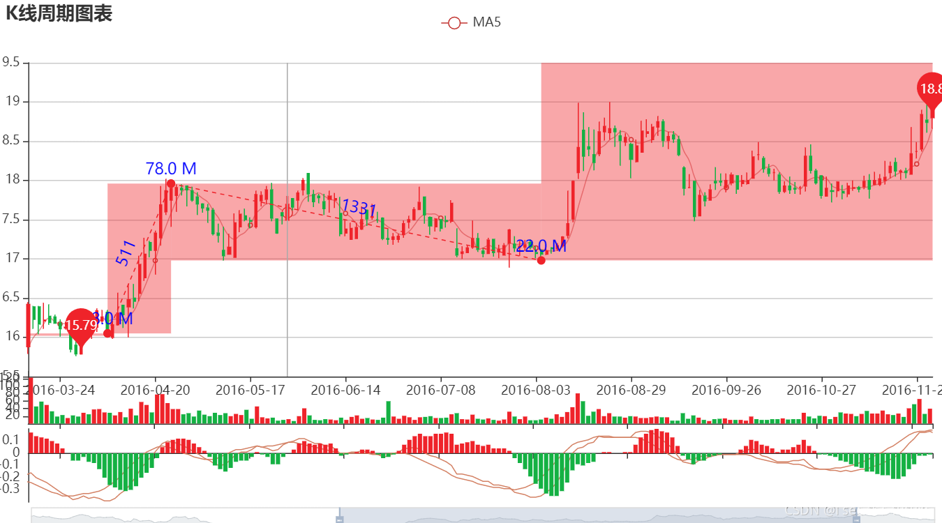
69.2 Candlestick - Kline_itemstyle
from pyecharts import options as opts
from pyecharts.charts import Kline

data = [
    [2320.26, 2320.26, 2287.3, 2362.94],
    [2300, 2291.3, 2288.26, 2308.38],
    [2295.35, 2346.5, 2295.35, 2345.92],
    [2347.22, 2358.98, 2337.35, 2363.8],
    [2360.75, 2382.48, 2347.89, 2383.76],
    [2383.43, 2385.42, 2371.23, 2391.82],
    [2377.41, 2419.02, 2369.57, 2421.15],
    [2425.92, 2428.15, 2417.58, 2440.38],
    [2411, 2433.13, 2403.3, 2437.42],
    [2432.68, 2334.48, 2427.7, 2441.73],
    [2430.69, 2418.53, 2394.22, 2433.89],
    [2416.62, 2432.4, 2414.4, 2443.03],
    [2441.91, 2421.56, 2418.43, 2444.8],
    [2420.26, 2382.91, 2373.53, 2427.07],
    [2383.49, 2397.18, 2370.61, 2397.94],
    [2378.82, 2325.95, 2309.17, 2378.82],
    [2322.94, 2314.16, 2308.76, 2330.88],
    [2320.62, 2325.82, 2315.01, 2338.78],
    [2313.74, 2293.34, 2289.89, 2340.71],
    [2297.77, 2313.22, 2292.03, 2324.63],
    [2322.32, 2365.59, 2308.92, 2366.16],
    [2364.54, 2359.51, 2330.86, 2369.65],
    [2332.08, 2273.4, 2259.25, 2333.54],
    [2274.81, 2326.31, 2270.1, 2328.14],
    [2333.61, 2347.18, 2321.6, 2351.44],
    [2340.44, 2324.29, 2304.27, 2352.02],
    [2326.42, 2318.61, 2314.59, 2333.67],
    [2314.68, 2310.59, 2296.58, 2320.96],
    [2309.16, 2286.6, 2264.83, 2333.29],
    [2282.17, 2263.97, 2253.25, 2286.33],
    [2255.77, 2270.28, 2253.31, 2276.22],
]


c = (
    Kline()
    .add_xaxis(["2017/7/{}".format(i + 1) for i in range(31)])
    .add_yaxis(
        "kline",
        data,
        itemstyle_opts=opts.ItemStyleOpts(
            color="#ec0000",
            color0="#00da3c",
            border_color="#8A0000",
            border_color0="#008F28",
        ),
    )
    .set_global_opts(
        xaxis_opts=opts.AxisOpts(is_scale=True),
        yaxis_opts=opts.AxisOpts(
            is_scale=True,
            splitarea_opts=opts.SplitAreaOpts(
                is_show=True, areastyle_opts=opts.AreaStyleOpts(opacity=1)
            ),
        ),
        datazoom_opts=[opts.DataZoomOpts(type_="inside")],
        title_opts=opts.TitleOpts(title="Kline-ItemStyle"),
    )
    .render("kline_itemstyle.html")
)
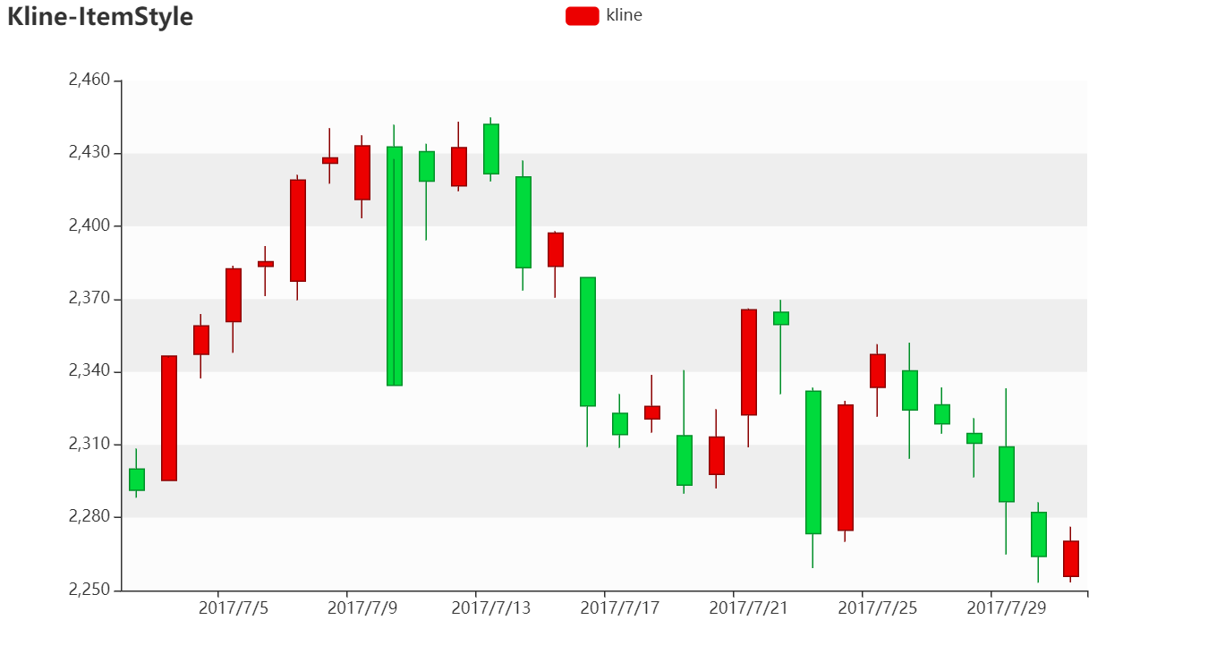
69.3 Candlestick - Basic_candlestick
import pyecharts.options as opts
from pyecharts.charts import Candlestick

x_data = ["2017-10-24", "2017-10-25", "2017-10-26", "2017-10-27"]
y_data = [[20, 30, 10, 35], [40, 35, 30, 55], [33, 38, 33, 40], [40, 40, 32, 42]]

(
    Candlestick(init_opts=opts.InitOpts(width="1440px", height="720px"))
    .add_xaxis(xaxis_data=x_data)
    .add_yaxis(series_name="", y_axis=y_data)
    .set_series_opts()
    .set_global_opts(
        yaxis_opts=opts.AxisOpts(
            splitline_opts=opts.SplitLineOpts(
                is_show=True, linestyle_opts=opts.LineStyleOpts(width=1)
            )
        )
    )
    .render("basic_candlestick.html")
)
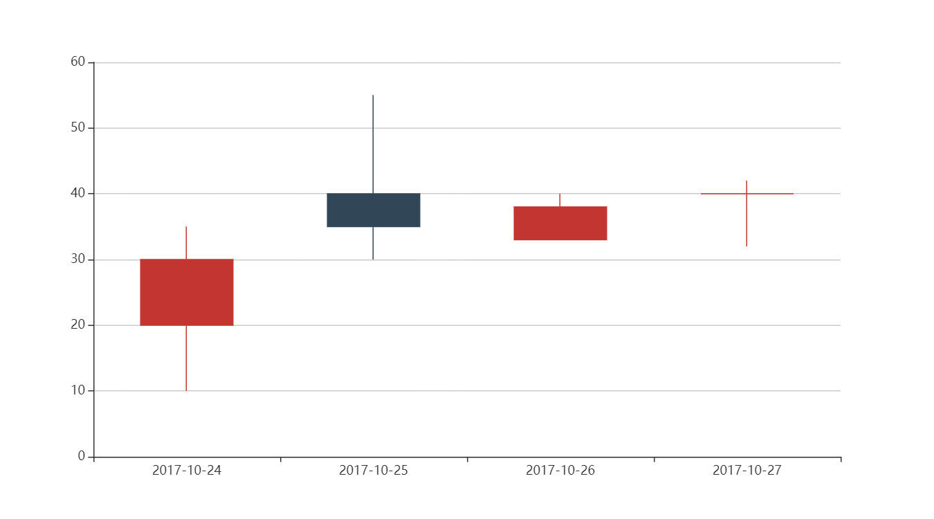
69.4 Candlestick - Kline_markline
from pyecharts import options as opts
from pyecharts.charts import Kline

data = [
    [2320.26, 2320.26, 2287.3, 2362.94],
    [2300, 2291.3, 2288.26, 2308.38],
    [2295.35, 2346.5, 2295.35, 2345.92],
    [2347.22, 2358.98, 2337.35, 2363.8],
    [2360.75, 2382.48, 2347.89, 2383.76],
    [2383.43, 2385.42, 2371.23, 2391.82],
    [2377.41, 2419.02, 2369.57, 2421.15],
    [2425.92, 2428.15, 2417.58, 2440.38],
    [2411, 2433.13, 2403.3, 2437.42],
    [2432.68, 2334.48, 2427.7, 2441.73],
    [2430.69, 2418.53, 2394.22, 2433.89],
    [2416.62, 2432.4, 2414.4, 2443.03],
    [2441.91, 2421.56, 2418.43, 2444.8],
    [2420.26, 2382.91, 2373.53, 2427.07],
    [2383.49, 2397.18, 2370.61, 2397.94],
    [2378.82, 2325.95, 2309.17, 2378.82],
    [2322.94, 2314.16, 2308.76, 2330.88],
    [2320.62, 2325.82, 2315.01, 2338.78],
    [2313.74, 2293.34, 2289.89, 2340.71],
    [2297.77, 2313.22, 2292.03, 2324.63],
    [2322.32, 2365.59, 2308.92, 2366.16],
    [2364.54, 2359.51, 2330.86, 2369.65],
    [2332.08, 2273.4, 2259.25, 2333.54],
    [2274.81, 2326.31, 2270.1, 2328.14],
    [2333.61, 2347.18, 2321.6, 2351.44],
    [2340.44, 2324.29, 2304.27, 2352.02],
    [2326.42, 2318.61, 2314.59, 2333.67],
    [2314.68, 2310.59, 2296.58, 2320.96],
    [2309.16, 2286.6, 2264.83, 2333.29],
    [2282.17, 2263.97, 2253.25, 2286.33],
    [2255.77, 2270.28, 2253.31, 2276.22],
]

c = (
    Kline()
    .add_xaxis(["2017/7/{}".format(i + 1) for i in range(31)])
    .add_yaxis(
        "kline",
        data,
        markline_opts=opts.MarkLineOpts(
            data=[opts.MarkLineItem(type_="max", value_dim="close")]
        ),
    )
    .set_global_opts(
        xaxis_opts=opts.AxisOpts(is_scale=True),
        yaxis_opts=opts.AxisOpts(
            is_scale=True,
            splitarea_opts=opts.SplitAreaOpts(
                is_show=True, areastyle_opts=opts.AreaStyleOpts(opacity=1)
            ),
        ),
        title_opts=opts.TitleOpts(title="Kline-MarkLine"),
    )
    .render("kline_markline.html")
)
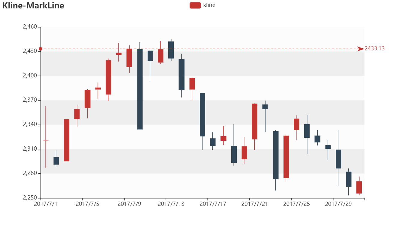
69.5 Candlestick - Kline_base
from pyecharts import options as opts
from pyecharts.charts import Kline

data = [
    [2320.26, 2320.26, 2287.3, 2362.94],
    [2300, 2291.3, 2288.26, 2308.38],
    [2295.35, 2346.5, 2295.35, 2345.92],
    [2347.22, 2358.98, 2337.35, 2363.8],
    [2360.75, 2382.48, 2347.89, 2383.76],
    [2383.43, 2385.42, 2371.23, 2391.82],
    [2377.41, 2419.02, 2369.57, 2421.15],
    [2425.92, 2428.15, 2417.58, 2440.38],
    [2411, 2433.13, 2403.3, 2437.42],
    [2432.68, 2334.48, 2427.7, 2441.73],
    [2430.69, 2418.53, 2394.22, 2433.89],
    [2416.62, 2432.4, 2414.4, 2443.03],
    [2441.91, 2421.56, 2418.43, 2444.8],
    [2420.26, 2382.91, 2373.53, 2427.07],
    [2383.49, 2397.18, 2370.61, 2397.94],
    [2378.82, 2325.95, 2309.17, 2378.82],
    [2322.94, 2314.16, 2308.76, 2330.88],
    [2320.62, 2325.82, 2315.01, 2338.78],
    [2313.74, 2293.34, 2289.89, 2340.71],
    [2297.77, 2313.22, 2292.03, 2324.63],
    [2322.32, 2365.59, 2308.92, 2366.16],
    [2364.54, 2359.51, 2330.86, 2369.65],
    [2332.08, 2273.4, 2259.25, 2333.54],
    [2274.81, 2326.31, 2270.1, 2328.14],
    [2333.61, 2347.18, 2321.6, 2351.44],
    [2340.44, 2324.29, 2304.27, 2352.02],
    [2326.42, 2318.61, 2314.59, 2333.67],
    [2314.68, 2310.59, 2296.58, 2320.96],
    [2309.16, 2286.6, 2264.83, 2333.29],
    [2282.17, 2263.97, 2253.25, 2286.33],
    [2255.77, 2270.28, 2253.31, 2276.22],
]


c = (
    Kline()
    .add_xaxis(["2017/7/{}".format(i + 1) for i in range(31)])
    .add_yaxis("kline", data)
    .set_global_opts(
        yaxis_opts=opts.AxisOpts(is_scale=True),
        xaxis_opts=opts.AxisOpts(is_scale=True),
        title_opts=opts.TitleOpts(title="Kline-基本示例"),
    )
    .render("kline_base.html")
)
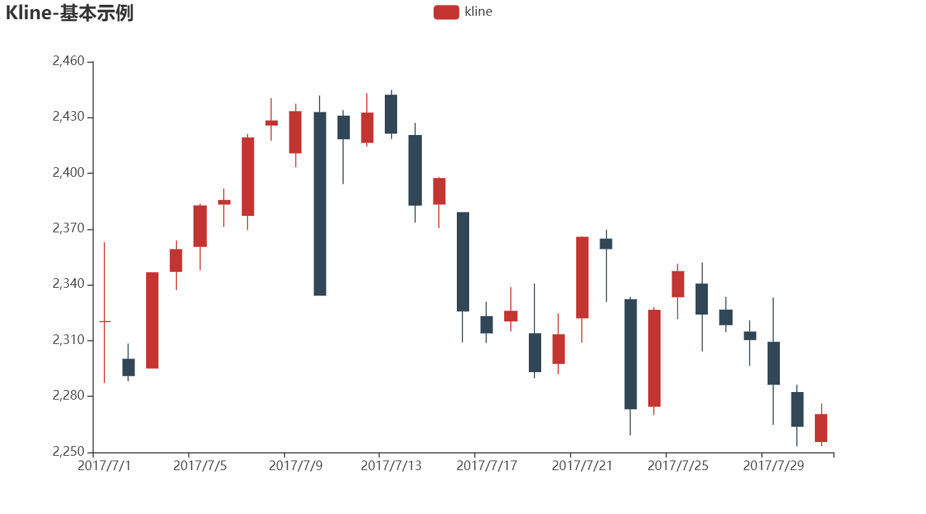
69.6 Candlestick - Kline_datazoom_inside
from pyecharts import options as opts
from pyecharts.charts import Kline

data = [
    [2320.26, 2320.26, 2287.3, 2362.94],
    [2300, 2291.3, 2288.26, 2308.38],
    [2295.35, 2346.5, 2295.35, 2345.92],
    [2347.22, 2358.98, 2337.35, 2363.8],
    [2360.75, 2382.48, 2347.89, 2383.76],
    [2383.43, 2385.42, 2371.23, 2391.82],
    [2377.41, 2419.02, 2369.57, 2421.15],
    [2425.92, 2428.15, 2417.58, 2440.38],
    [2411, 2433.13, 2403.3, 2437.42],
    [2432.68, 2334.48, 2427.7, 2441.73],
    [2430.69, 2418.53, 2394.22, 2433.89],
    [2416.62, 2432.4, 2414.4, 2443.03],
    [2441.91, 2421.56, 2418.43, 2444.8],
    [2420.26, 2382.91, 2373.53, 2427.07],
    [2383.49, 2397.18, 2370.61, 2397.94],
    [2378.82, 2325.95, 2309.17, 2378.82],
    [2322.94, 2314.16, 2308.76, 2330.88],
    [2320.62, 2325.82, 2315.01, 2338.78],
    [2313.74, 2293.34, 2289.89, 2340.71],
    [2297.77, 2313.22, 2292.03, 2324.63],
    [2322.32, 2365.59, 2308.92, 2366.16],
    [2364.54, 2359.51, 2330.86, 2369.65],
    [2332.08, 2273.4, 2259.25, 2333.54],
    [2274.81, 2326.31, 2270.1, 2328.14],
    [2333.61, 2347.18, 2321.6, 2351.44],
    [2340.44, 2324.29, 2304.27, 2352.02],
    [2326.42, 2318.61, 2314.59, 2333.67],
    [2314.68, 2310.59, 2296.58, 2320.96],
    [2309.16, 2286.6, 2264.83, 2333.29],
    [2282.17, 2263.97, 2253.25, 2286.33],
    [2255.77, 2270.28, 2253.31, 2276.22],
]

c = (
    Kline()
    .add_xaxis(["2017/7/{}".format(i + 1) for i in range(31)])
    .add_yaxis("kline", data)
    .set_global_opts(
        xaxis_opts=opts.AxisOpts(is_scale=True),
        yaxis_opts=opts.AxisOpts(
            is_scale=True,
            splitarea_opts=opts.SplitAreaOpts(
                is_show=True, areastyle_opts=opts.AreaStyleOpts(opacity=1)
            ),
        ),
        datazoom_opts=[opts.DataZoomOpts(type_="inside")],
        title_opts=opts.TitleOpts(title="Kline-DataZoom-inside"),
    )
    .render("kline_datazoom_inside.html")
)
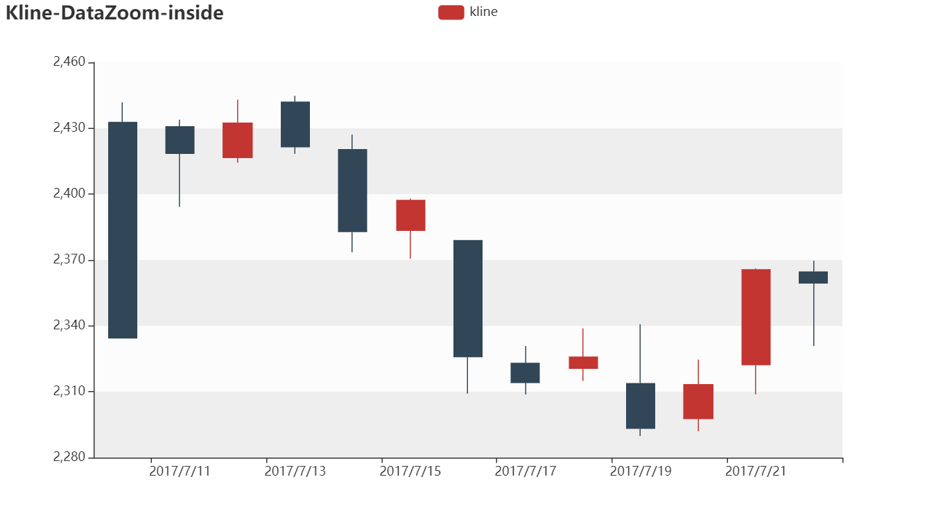
69.7 Candlestick - Kline_datazoom_slider_position
from pyecharts import options as opts
from pyecharts.charts import Kline

data = [
    [2320.26, 2320.26, 2287.3, 2362.94],
    [2300, 2291.3, 2288.26, 2308.38],
    [2295.35, 2346.5, 2295.35, 2345.92],
    [2347.22, 2358.98, 2337.35, 2363.8],
    [2360.75, 2382.48, 2347.89, 2383.76],
    [2383.43, 2385.42, 2371.23, 2391.82],
    [2377.41, 2419.02, 2369.57, 2421.15],
    [2425.92, 2428.15, 2417.58, 2440.38],
    [2411, 2433.13, 2403.3, 2437.42],
    [2432.68, 2334.48, 2427.7, 2441.73],
    [2430.69, 2418.53, 2394.22, 2433.89],
    [2416.62, 2432.4, 2414.4, 2443.03],
    [2441.91, 2421.56, 2418.43, 2444.8],
    [2420.26, 2382.91, 2373.53, 2427.07],
    [2383.49, 2397.18, 2370.61, 2397.94],
    [2378.82, 2325.95, 2309.17, 2378.82],
    [2322.94, 2314.16, 2308.76, 2330.88],
    [2320.62, 2325.82, 2315.01, 2338.78],
    [2313.74, 2293.34, 2289.89, 2340.71],
    [2297.77, 2313.22, 2292.03, 2324.63],
    [2322.32, 2365.59, 2308.92, 2366.16],
    [2364.54, 2359.51, 2330.86, 2369.65],
    [2332.08, 2273.4, 2259.25, 2333.54],
    [2274.81, 2326.31, 2270.1, 2328.14],
    [2333.61, 2347.18, 2321.6, 2351.44],
    [2340.44, 2324.29, 2304.27, 2352.02],
    [2326.42, 2318.61, 2314.59, 2333.67],
    [2314.68, 2310.59, 2296.58, 2320.96],
    [2309.16, 2286.6, 2264.83, 2333.29],
    [2282.17, 2263.97, 2253.25, 2286.33],
    [2255.77, 2270.28, 2253.31, 2276.22],
]

c = (
    Kline()
    .add_xaxis(["2017/7/{}".format(i + 1) for i in range(31)])
    .add_yaxis("kline", data)
    .set_global_opts(
        xaxis_opts=opts.AxisOpts(is_scale=True),
        yaxis_opts=opts.AxisOpts(
            is_scale=True,
            splitarea_opts=opts.SplitAreaOpts(
                is_show=True, areastyle_opts=opts.AreaStyleOpts(opacity=1)
            ),
        ),
        datazoom_opts=[opts.DataZoomOpts(pos_bottom="-2%")],
        title_opts=opts.TitleOpts(title="Kline-DataZoom-slider-Position"),
    )
    .render("kline_datazoom_slider_position.html")
)
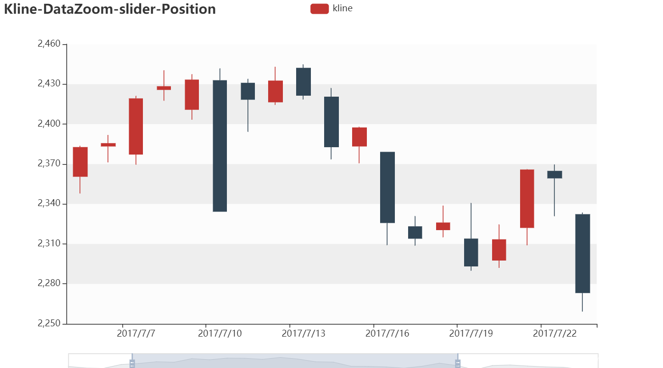
?69.8 Candlestick - Professional_kline_brush
import requests
from typing import List, Union

from pyecharts import options as opts
from pyecharts.charts import Kline, Line, Bar, Grid


def get_data():
    response = requests.get(
        url="https://echarts.apache.org/examples/data/asset/data/stock-DJI.json"
    )
    json_response = response.json()
    # 解析数据
    return split_data(data=json_response)


def split_data(data):
    category_data = []
    values = []
    volumes = []

    for i, tick in enumerate(data):
        category_data.append(tick[0])
        values.append(tick)
        volumes.append([i, tick[4], 1 if tick[1] > tick[2] else -1])
    return {"categoryData": category_data, "values": values, "volumes": volumes}


def calculate_ma(day_count: int, data):
    result: List[Union[float, str]] = []
    for i in range(len(data["values"])):
        if i < day_count:
            result.append("-")
            continue
        sum_total = 0.0
        for j in range(day_count):
            sum_total += float(data["values"][i - j][1])
        result.append(abs(float("%.3f" % (sum_total / day_count))))
    return result


def draw_charts():
    kline_data = [data[1:-1] for data in chart_data["values"]]
    kline = (
        Kline()
        .add_xaxis(xaxis_data=chart_data["categoryData"])
        .add_yaxis(
            series_name="Dow-Jones index",
            y_axis=kline_data,
            itemstyle_opts=opts.ItemStyleOpts(color="#ec0000", color0="#00da3c"),
        )
        .set_global_opts(
            legend_opts=opts.LegendOpts(
                is_show=False, pos_bottom=10, pos_left="center"
            ),
            datazoom_opts=[
                opts.DataZoomOpts(
                    is_show=False,
                    type_="inside",
                    xaxis_index=[0, 1],
                    range_start=98,
                    range_end=100,
                ),
                opts.DataZoomOpts(
                    is_show=True,
                    xaxis_index=[0, 1],
                    type_="slider",
                    pos_top="85%",
                    range_start=98,
                    range_end=100,
                ),
            ],
            yaxis_opts=opts.AxisOpts(
                is_scale=True,
                splitarea_opts=opts.SplitAreaOpts(
                    is_show=True, areastyle_opts=opts.AreaStyleOpts(opacity=1)
                ),
            ),
            tooltip_opts=opts.TooltipOpts(
                trigger="axis",
                axis_pointer_type="cross",
                background_color="rgba(245, 245, 245, 0.8)",
                border_width=1,
                border_color="#ccc",
                textstyle_opts=opts.TextStyleOpts(color="#000"),
            ),
            visualmap_opts=opts.VisualMapOpts(
                is_show=False,
                dimension=2,
                series_index=5,
                is_piecewise=True,
                pieces=[
                    {"value": 1, "color": "#00da3c"},
                    {"value": -1, "color": "#ec0000"},
                ],
            ),
            axispointer_opts=opts.AxisPointerOpts(
                is_show=True,
                link=[{"xAxisIndex": "all"}],
                label=opts.LabelOpts(background_color="#777"),
            ),
            brush_opts=opts.BrushOpts(
                x_axis_index="all",
                brush_link="all",
                out_of_brush={"colorAlpha": 0.1},
                brush_type="lineX",
            ),
        )
    )

    line = (
        Line()
        .add_xaxis(xaxis_data=chart_data["categoryData"])
        .add_yaxis(
            series_name="MA5",
            y_axis=calculate_ma(day_count=5, data=chart_data),
            is_smooth=True,
            is_hover_animation=False,
            linestyle_opts=opts.LineStyleOpts(width=3, opacity=0.5),
            label_opts=opts.LabelOpts(is_show=False),
        )
        .add_yaxis(
            series_name="MA10",
            y_axis=calculate_ma(day_count=10, data=chart_data),
            is_smooth=True,
            is_hover_animation=False,
            linestyle_opts=opts.LineStyleOpts(width=3, opacity=0.5),
            label_opts=opts.LabelOpts(is_show=False),
        )
        .add_yaxis(
            series_name="MA20",
            y_axis=calculate_ma(day_count=20, data=chart_data),
            is_smooth=True,
            is_hover_animation=False,
            linestyle_opts=opts.LineStyleOpts(width=3, opacity=0.5),
            label_opts=opts.LabelOpts(is_show=False),
        )
        .add_yaxis(
            series_name="MA30",
            y_axis=calculate_ma(day_count=30, data=chart_data),
            is_smooth=True,
            is_hover_animation=False,
            linestyle_opts=opts.LineStyleOpts(width=3, opacity=0.5),
            label_opts=opts.LabelOpts(is_show=False),
        )
        .set_global_opts(xaxis_opts=opts.AxisOpts(type_="category"))
    )

    bar = (
        Bar()
        .add_xaxis(xaxis_data=chart_data["categoryData"])
        .add_yaxis(
            series_name="Volume",
            y_axis=chart_data["volumes"],
            xaxis_index=1,
            yaxis_index=1,
            label_opts=opts.LabelOpts(is_show=False),
        )
        .set_global_opts(
            xaxis_opts=opts.AxisOpts(
                type_="category",
                is_scale=True,
                grid_index=1,
                boundary_gap=False,
                axisline_opts=opts.AxisLineOpts(is_on_zero=False),
                axistick_opts=opts.AxisTickOpts(is_show=False),
                splitline_opts=opts.SplitLineOpts(is_show=False),
                axislabel_opts=opts.LabelOpts(is_show=False),
                split_number=20,
                min_="dataMin",
                max_="dataMax",
            ),
            yaxis_opts=opts.AxisOpts(
                grid_index=1,
                is_scale=True,
                split_number=2,
                axislabel_opts=opts.LabelOpts(is_show=False),
                axisline_opts=opts.AxisLineOpts(is_show=False),
                axistick_opts=opts.AxisTickOpts(is_show=False),
                splitline_opts=opts.SplitLineOpts(is_show=False),
            ),
            legend_opts=opts.LegendOpts(is_show=False),
        )
    )

    # Kline And Line
    overlap_kline_line = kline.overlap(line)

    # Grid Overlap + Bar
    grid_chart = Grid(
        init_opts=opts.InitOpts(
            width="1000px",
            height="800px",
            animation_opts=opts.AnimationOpts(animation=False),
        )
    )
    grid_chart.add(
        overlap_kline_line,
        grid_opts=opts.GridOpts(pos_left="10%", pos_right="8%", height="50%"),
    )
    grid_chart.add(
        bar,
        grid_opts=opts.GridOpts(
            pos_left="10%", pos_right="8%", pos_top="63%", height="16%"
        ),
    )

    grid_chart.render("professional_kline_brush.html")


if __name__ == "__main__":
    chart_data = get_data()
    draw_charts()
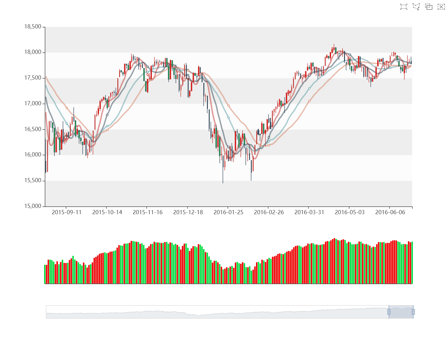
69.9 Candlestick - Kline_datazoom_slider
from pyecharts import options as opts
from pyecharts.charts import Kline

data = [
    [2320.26, 2320.26, 2287.3, 2362.94],
    [2300, 2291.3, 2288.26, 2308.38],
    [2295.35, 2346.5, 2295.35, 2345.92],
    [2347.22, 2358.98, 2337.35, 2363.8],
    [2360.75, 2382.48, 2347.89, 2383.76],
    [2383.43, 2385.42, 2371.23, 2391.82],
    [2377.41, 2419.02, 2369.57, 2421.15],
    [2425.92, 2428.15, 2417.58, 2440.38],
    [2411, 2433.13, 2403.3, 2437.42],
    [2432.68, 2334.48, 2427.7, 2441.73],
    [2430.69, 2418.53, 2394.22, 2433.89],
    [2416.62, 2432.4, 2414.4, 2443.03],
    [2441.91, 2421.56, 2418.43, 2444.8],
    [2420.26, 2382.91, 2373.53, 2427.07],
    [2383.49, 2397.18, 2370.61, 2397.94],
    [2378.82, 2325.95, 2309.17, 2378.82],
    [2322.94, 2314.16, 2308.76, 2330.88],
    [2320.62, 2325.82, 2315.01, 2338.78],
    [2313.74, 2293.34, 2289.89, 2340.71],
    [2297.77, 2313.22, 2292.03, 2324.63],
    [2322.32, 2365.59, 2308.92, 2366.16],
    [2364.54, 2359.51, 2330.86, 2369.65],
    [2332.08, 2273.4, 2259.25, 2333.54],
    [2274.81, 2326.31, 2270.1, 2328.14],
    [2333.61, 2347.18, 2321.6, 2351.44],
    [2340.44, 2324.29, 2304.27, 2352.02],
    [2326.42, 2318.61, 2314.59, 2333.67],
    [2314.68, 2310.59, 2296.58, 2320.96],
    [2309.16, 2286.6, 2264.83, 2333.29],
    [2282.17, 2263.97, 2253.25, 2286.33],
    [2255.77, 2270.28, 2253.31, 2276.22],
]

c = (
    Kline()
    .add_xaxis(["2017/7/{}".format(i + 1) for i in range(31)])
    .add_yaxis("kline", data)
    .set_global_opts(
        xaxis_opts=opts.AxisOpts(is_scale=True),
        yaxis_opts=opts.AxisOpts(
            is_scale=True,
            splitarea_opts=opts.SplitAreaOpts(
                is_show=True, areastyle_opts=opts.AreaStyleOpts(opacity=1)
            ),
        ),
        datazoom_opts=[opts.DataZoomOpts()],
        title_opts=opts.TitleOpts(title="Kline-DataZoom-slider"),
    )
    .render("kline_datazoom_slider.html")
)
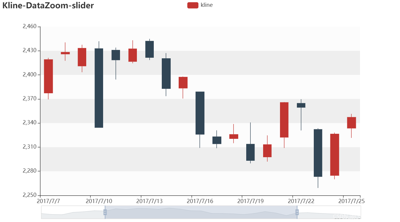
69.10 Candlestick - Kline_split_area
from pyecharts import options as opts
from pyecharts.charts import Kline

data = [
    [2320.26, 2320.26, 2287.3, 2362.94],
    [2300, 2291.3, 2288.26, 2308.38],
    [2295.35, 2346.5, 2295.35, 2345.92],
    [2347.22, 2358.98, 2337.35, 2363.8],
    [2360.75, 2382.48, 2347.89, 2383.76],
    [2383.43, 2385.42, 2371.23, 2391.82],
    [2377.41, 2419.02, 2369.57, 2421.15],
    [2425.92, 2428.15, 2417.58, 2440.38],
    [2411, 2433.13, 2403.3, 2437.42],
    [2432.68, 2334.48, 2427.7, 2441.73],
    [2430.69, 2418.53, 2394.22, 2433.89],
    [2416.62, 2432.4, 2414.4, 2443.03],
    [2441.91, 2421.56, 2418.43, 2444.8],
    [2420.26, 2382.91, 2373.53, 2427.07],
    [2383.49, 2397.18, 2370.61, 2397.94],
    [2378.82, 2325.95, 2309.17, 2378.82],
    [2322.94, 2314.16, 2308.76, 2330.88],
    [2320.62, 2325.82, 2315.01, 2338.78],
    [2313.74, 2293.34, 2289.89, 2340.71],
    [2297.77, 2313.22, 2292.03, 2324.63],
    [2322.32, 2365.59, 2308.92, 2366.16],
    [2364.54, 2359.51, 2330.86, 2369.65],
    [2332.08, 2273.4, 2259.25, 2333.54],
    [2274.81, 2326.31, 2270.1, 2328.14],
    [2333.61, 2347.18, 2321.6, 2351.44],
    [2340.44, 2324.29, 2304.27, 2352.02],
    [2326.42, 2318.61, 2314.59, 2333.67],
    [2314.68, 2310.59, 2296.58, 2320.96],
    [2309.16, 2286.6, 2264.83, 2333.29],
    [2282.17, 2263.97, 2253.25, 2286.33],
    [2255.77, 2270.28, 2253.31, 2276.22],
]


c = (
    Kline()
    .add_xaxis(["2017/7/{}".format(i + 1) for i in range(31)])
    .add_yaxis("kline", data)
    .set_global_opts(
        xaxis_opts=opts.AxisOpts(is_scale=True),
        yaxis_opts=opts.AxisOpts(
            is_scale=True,
            splitarea_opts=opts.SplitAreaOpts(
                is_show=True, areastyle_opts=opts.AreaStyleOpts(opacity=1)
            ),
        ),
        title_opts=opts.TitleOpts(title="Kline-显示分割区域"),
    )
    .render("kline_split_area.html")
)
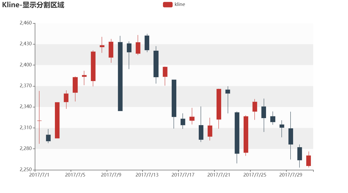
69.11 Season实践:Candlestick–yaxis_opts=opts.AxisOpts(is_scale=True)
is_scale=True是显示局部重要的坐标轴,is_scale=False是显示全部的坐标轴
 .set_global_opts(
            xaxis_opts=opts.AxisOpts(is_scale=True),
            yaxis_opts=opts.AxisOpts(is_scale=False)
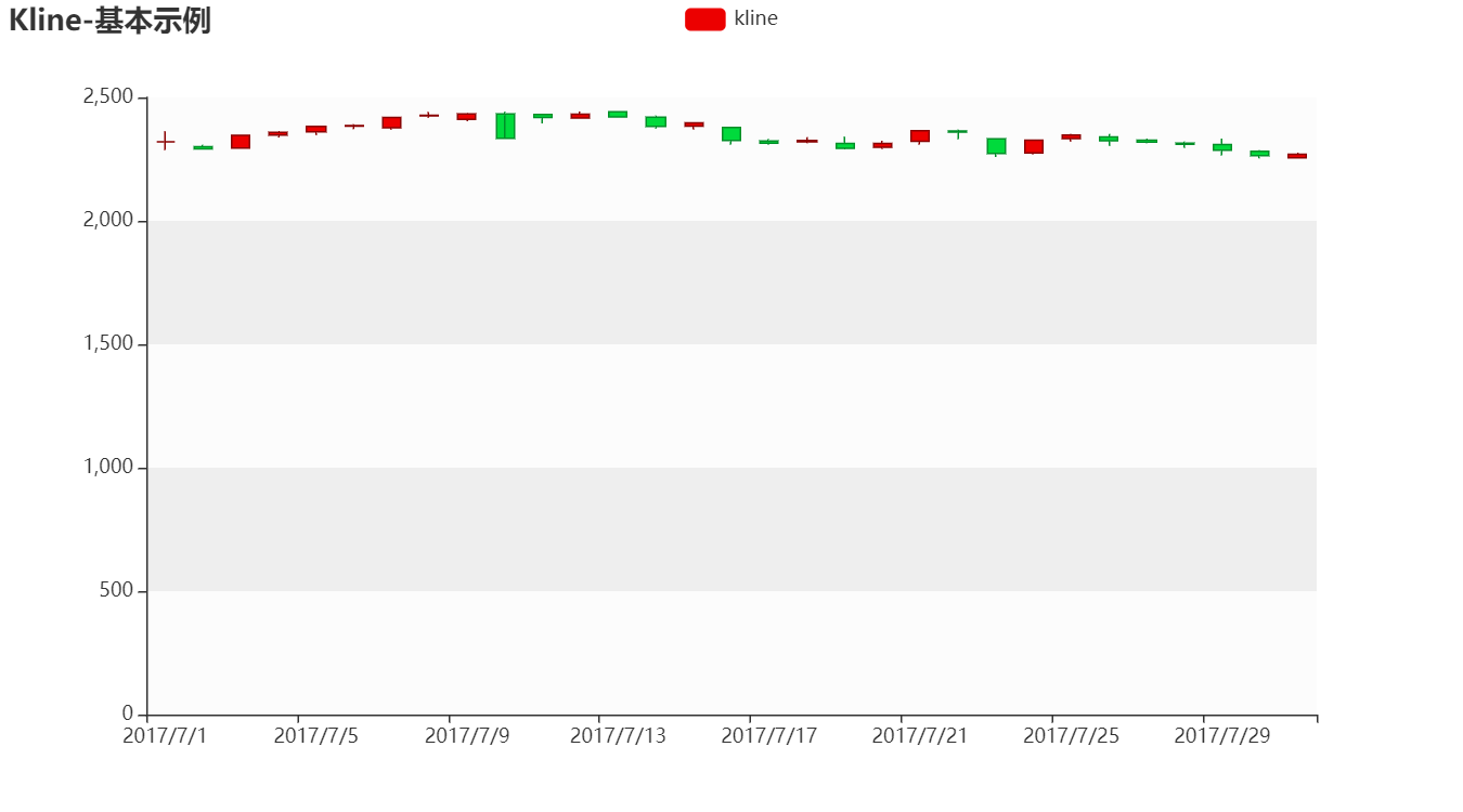
 .set_global_opts(
            xaxis_opts=opts.AxisOpts(is_scale=True),
            yaxis_opts=opts.AxisOpts(is_scale=True)
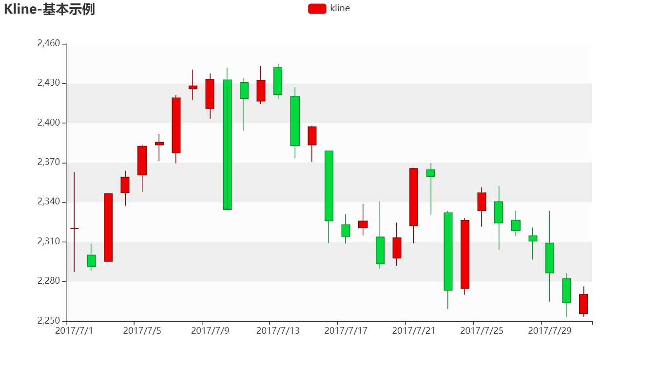
- 完整代码如下
def Kline_base():
    data = [
        [2320.26, 2320.26, 2287.3, 2362.94],
        [2300, 2291.3, 2288.26, 2308.38],
        [2295.35, 2346.5, 2295.35, 2345.92],
        [2347.22, 2358.98, 2337.35, 2363.8],
        [2360.75, 2382.48, 2347.89, 2383.76],
        [2383.43, 2385.42, 2371.23, 2391.82],
        [2377.41, 2419.02, 2369.57, 2421.15],
        [2425.92, 2428.15, 2417.58, 2440.38],
        [2411, 2433.13, 2403.3, 2437.42],
        [2432.68, 2334.48, 2427.7, 2441.73],
        [2430.69, 2418.53, 2394.22, 2433.89],
        [2416.62, 2432.4, 2414.4, 2443.03],
        [2441.91, 2421.56, 2418.43, 2444.8],
        [2420.26, 2382.91, 2373.53, 2427.07],
        [2383.49, 2397.18, 2370.61, 2397.94],
        [2378.82, 2325.95, 2309.17, 2378.82],
        [2322.94, 2314.16, 2308.76, 2330.88],
        [2320.62, 2325.82, 2315.01, 2338.78],
        [2313.74, 2293.34, 2289.89, 2340.71],
        [2297.77, 2313.22, 2292.03, 2324.63],
        [2322.32, 2365.59, 2308.92, 2366.16],
        [2364.54, 2359.51, 2330.86, 2369.65],
        [2332.08, 2273.4, 2259.25, 2333.54],
        [2274.81, 2326.31, 2270.1, 2328.14],
        [2333.61, 2347.18, 2321.6, 2351.44],
        [2340.44, 2324.29, 2304.27, 2352.02],
        [2326.42, 2318.61, 2314.59, 2333.67],
        [2314.68, 2310.59, 2296.58, 2320.96],
        [2309.16, 2286.6, 2264.83, 2333.29],
        [2282.17, 2263.97, 2253.25, 2286.33],
        [2255.77, 2270.28, 2253.31, 2276.22],
    ]

    c = (
        Kline()
        .add_xaxis(["2017/7/{}".format(i + 1) for i in range(31)])
        .add_yaxis("kline",
                data,
                itemstyle_opts=opts.ItemStyleOpts(
                color="#ec0000",
                color0="#00da3c",
                border_color="#8A0000",
                border_color0="#008F28",
                ),
        )
        .set_global_opts(
            xaxis_opts=opts.AxisOpts(is_scale=True),
            yaxis_opts=opts.AxisOpts(is_scale=False,splitarea_opts=opts.SplitAreaOpts(is_show=True, areastyle_opts=opts.AreaStyleOpts(opacity=1))),
            title_opts=opts.TitleOpts(title="Kline-基本示例"),
        )
        #.render("kline_base.html")
    )
    return c
70.Line:折线/面积图
- class pyecharts.charts.Line(RectChart)
class Line(
    # 初始化配置项,参考 `global_options.InitOpts`
    init_opts: opts.InitOpts = opts.InitOpts()
)
- func pyecharts.charts.Line.add_yaxis
def add_yaxis(
    # 系列名称,用于 tooltip 的显示,legend 的图例筛选。
    series_name: str,

    # 系列数据
    y_axis: types.Sequence[types.Union[opts.LineItem, dict]],

    # 是否选中图例
    is_selected: bool = True,

    # 是否连接空数据,空数据使用 `None` 填充
    is_connect_nones: bool = False,

    # 使用的 x 轴的 index,在单个图表实例中存在多个 x 轴的时候有用。
    xaxis_index: Optional[Numeric] = None,

    # 使用的 y 轴的 index,在单个图表实例中存在多个 y 轴的时候有用。
    yaxis_index: Optional[Numeric] = None,

    # 系列 label 颜色
    color: Optional[str] = None,

    # 是否显示 symbol, 如果 false 则只有在 tooltip hover 的时候显示。
    is_symbol_show: bool = True,

    # 标记的图形。
    # ECharts 提供的标记类型包括 'circle', 'rect', 'roundRect', 'triangle',
    # 'diamond', 'pin', 'arrow', 'none'
    # 可以通过 'image://url' 设置为图片,其中 URL 为图片的链接,或者 dataURI。
    symbol: Optional[str] = None,

    # 标记的大小,可以设置成诸如 10 这样单一的数字,也可以用数组分开表示宽和高,
    # 例如 [20, 10] 表示标记宽为 20,高为 10。
    symbol_size: Union[Numeric, Sequence] = 4,

    # 数据堆叠,同个类目轴上系列配置相同的 stack 值可以堆叠放置。
    stack: Optional[str] = None,

    # 是否平滑曲线
    is_smooth: bool = False,

    # 是否裁剪超出坐标系部分的图形。折线图:裁掉所有超出坐标系的折线部分,拐点图形的逻辑按照散点图处理
    is_clip: bool = True,

    # 是否显示成阶梯图
    is_step: bool = False,

    # 是否开启 hover 在拐点标志上的提示动画效果。
    is_hover_animation: bool = True,

    # 折线图所有图形的 zlevel 值。
    # zlevel用于 Canvas 分层,不同zlevel值的图形会放置在不同的 Canvas 中,Canvas 分层是一种常见的优化手段。
    # zlevel 大的 Canvas 会放在 zlevel 小的 Canvas 的上面。
    z_level: types.Numeric = 0,

    # 折线图组件的所有图形的z值。控制图形的前后顺序。z值小的图形会被z值大的图形覆盖。
    # z 相比 zlevel 优先级更低,而且不会创建新的 Canvas。
    z: types.Numeric = 0,

    # 标记点配置项,参考 `series_options.MarkPointOpts`
    markpoint_opts: Union[opts.MarkPointOpts, dict, None] = None,

    # 标记线配置项,参考 `series_options.MarkLineOpts`
    markline_opts: Union[opts.MarkLineOpts, dict, None] = None,

    # 提示框组件配置项,参考 `series_options.TooltipOpts`
    tooltip_opts: Union[opts.TooltipOpts, dict, None] = None,

    # 标签配置项,参考 `series_options.LabelOpts`
    label_opts: Union[opts.LabelOpts, dict] = opts.LabelOpts(),

    # 线样式配置项,参考 `series_options.LineStyleOpts`
    linestyle_opts: Union[opts.LineStyleOpts, dict] = opts.LineStyleOpts(),

    # 填充区域配置项,参考 `series_options.AreaStyleOpts`
    areastyle_opts: Union[opts.AreaStyleOpts, dict] = opts.AreaStyleOpts(),

    # 图元样式配置项,参考 `series_options.ItemStyleOpts`
    itemstyle_opts: Union[opts.ItemStyleOpts, dict, None] = None,
)
- LineItem:折线图数据项
class LineItem(
    # 数据项名称。
    name: Union[str, Numeric] = None,

    # 数据项的值
    value: Union[str, Numeric] = None,

    # 单个数据标记的图形。
    symbol: Optional[str] = None,

    # 单个数据标记的大小
    symbol_size: Union[Sequence[Numeric], Numeric] = None,

    # 单个数据标记的旋转角度(而非弧度)。
    symbol_rotate: Optional[Numeric] = None,

    # 如果 symbol 是 path:// 的形式,是否在缩放时保持该图形的长宽比。
    symbol_keep_aspect: bool = False,

    # 单个数据标记相对于原本位置的偏移。
    symbol_offset: Optional[Sequence] = None,

    # 标签配置项,参考 `series_options.LabelOpts`
    label_opts: Union[LabelOpts, dict, None] = None,

    # 图元样式配置项,参考 `series_options.ItemStyleOpts`
    itemstyle_opts: Union[ItemStyleOpts, dict, None] = None,

    # 提示框组件配置项,参考 `series_options.TooltipOpts`
    tooltip_opts: Union[TooltipOpts, dict, None] = None,
)
70.1 Line - Temperature_change_line_chart
import pyecharts.options as opts
from pyecharts.charts import Line

"""
Gallery 使用 pyecharts 1.1.0
参考地址: https://www.echartsjs.com/examples/editor.html?c=line-marker

目前无法实现的功能:

1、最低气温的最高值暂时无法和 Echarts 的示例完全复刻
"""

week_name_list = ["周一", "周二", "周三", "周四", "周五", "周六", "周日"]
high_temperature = [11, 11, 15, 13, 12, 13, 10]
low_temperature = [1, -2, 2, 5, 3, 2, 0]


(
    Line(init_opts=opts.InitOpts(width="1600px", height="800px"))
    .add_xaxis(xaxis_data=week_name_list)
    .add_yaxis(
        series_name="最高气温",
        y_axis=high_temperature,
        markpoint_opts=opts.MarkPointOpts(
            data=[
                opts.MarkPointItem(type_="max", name="最大值"),
                opts.MarkPointItem(type_="min", name="最小值"),
            ]
        ),
        markline_opts=opts.MarkLineOpts(
            data=[opts.MarkLineItem(type_="average", name="平均值")]
        ),
    )
    .add_yaxis(
        series_name="最低气温",
        y_axis=low_temperature,
        markpoint_opts=opts.MarkPointOpts(
            data=[opts.MarkPointItem(value=-2, name="周最低", x=1, y=-1.5)]
        ),
        markline_opts=opts.MarkLineOpts(
            data=[
                opts.MarkLineItem(type_="average", name="平均值"),
                opts.MarkLineItem(symbol="none", x="90%", y="max"),
                opts.MarkLineItem(symbol="circle", type_="max", name="最高点"),
            ]
        ),
    )
    .set_global_opts(
        title_opts=opts.TitleOpts(title="未来一周气温变化", subtitle="纯属虚构"),
        tooltip_opts=opts.TooltipOpts(trigger="axis"),
        toolbox_opts=opts.ToolboxOpts(is_show=True),
        xaxis_opts=opts.AxisOpts(type_="category", boundary_gap=False),
    )
    .render("temperature_change_line_chart.html")
)
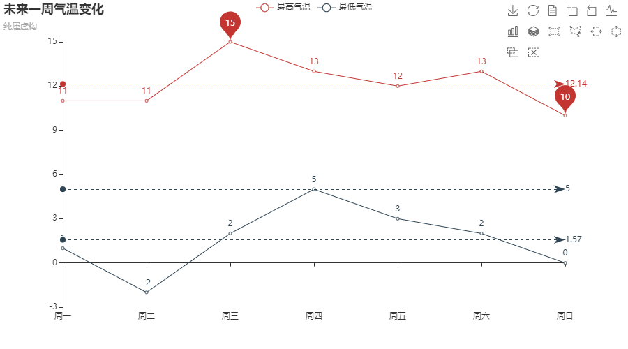
70.2 Line - Line_areastyle_boundary_gap
import pyecharts.options as opts
from pyecharts.charts import Line
from pyecharts.faker import Faker


c = (
    Line()
    .add_xaxis(Faker.choose())
    .add_yaxis("商家A", Faker.values(), is_smooth=True)
    .add_yaxis("商家B", Faker.values(), is_smooth=True)
    .set_series_opts(
        areastyle_opts=opts.AreaStyleOpts(opacity=0.5),
        label_opts=opts.LabelOpts(is_show=False),
    )
    .set_global_opts(
        title_opts=opts.TitleOpts(title="Line-面积图(紧贴 Y 轴)"),
        xaxis_opts=opts.AxisOpts(
            axistick_opts=opts.AxisTickOpts(is_align_with_label=True),
            is_scale=False,
            boundary_gap=False,
        ),
    )
    .render("line_areastyle_boundary_gap.html")
)
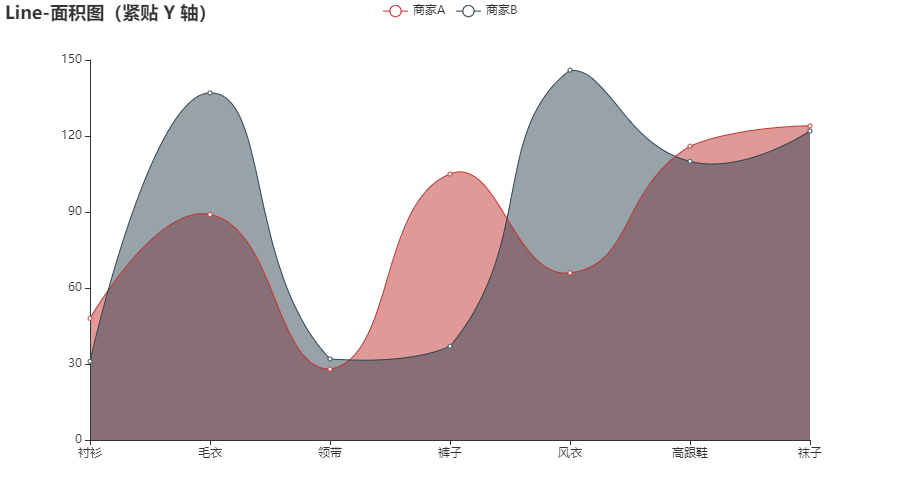
70.3 Line - Basic_line_chart
import pyecharts.options as opts
from pyecharts.charts import Line

"""
Gallery 使用 pyecharts 1.1.0
参考地址: https://echarts.apache.org/examples/editor.html?c=line-simple

目前无法实现的功能:

暂无
"""


x_data = ["Mon", "Tue", "Wed", "Thu", "Fri", "Sat", "Sun"]
y_data = [820, 932, 901, 934, 1290, 1330, 1320]


(
    Line()
    .set_global_opts(
        tooltip_opts=opts.TooltipOpts(is_show=False),
        xaxis_opts=opts.AxisOpts(type_="category"),
        yaxis_opts=opts.AxisOpts(
            type_="value",
            axistick_opts=opts.AxisTickOpts(is_show=True),
            splitline_opts=opts.SplitLineOpts(is_show=True),
        ),
    )
    .add_xaxis(xaxis_data=x_data)
    .add_yaxis(
        series_name="",
        y_axis=y_data,
        symbol="emptyCircle",
        is_symbol_show=True,
        label_opts=opts.LabelOpts(is_show=False),
    )
    .render("basic_line_chart.html")
)
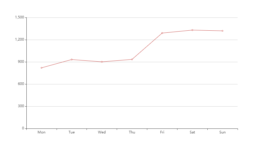
70.4 Line - Line_connect_null
import pyecharts.options as opts
from pyecharts.charts import Line
from pyecharts.faker import Faker

y = Faker.values()
y[3], y[5] = None, None
c = (
    Line()
    .add_xaxis(Faker.choose())
    .add_yaxis("商家A", y, is_connect_nones=True)
    .set_global_opts(title_opts=opts.TitleOpts(title="Line-连接空数据"))
    .render("line_connect_null.html")
)
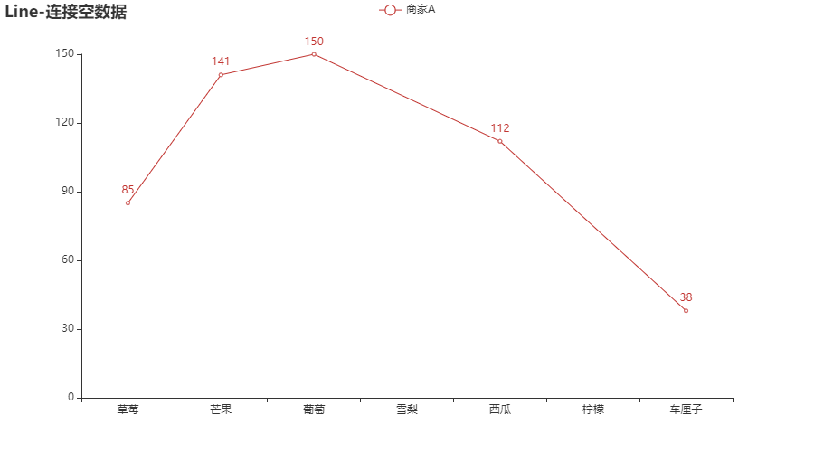
70.5 Line - Log_axis
import pyecharts.options as opts
from pyecharts.charts import Line

"""
Gallery 使用 pyecharts 1.1.0
参考地址: https://www.echartsjs.com/examples/editor.html?c=line-log

目前无法实现的功能:

1、暂无
"""

x_data = ["一", "二", "三", "四", "五", "六", "七", "八", "九"]
y_data_3 = [1, 3, 9, 27, 81, 247, 741, 2223, 6669]
y_data_2 = [1, 2, 4, 8, 16, 32, 64, 128, 256]
y_data_05 = [1 / 2, 1 / 4, 1 / 8, 1 / 16, 1 / 32, 1 / 64, 1 / 128, 1 / 256, 1 / 512]


(
    Line(init_opts=opts.InitOpts(width="1600px", height="800px"))
    .add_xaxis(xaxis_data=x_data)
    .add_yaxis(
        series_name="1/2的指数",
        y_axis=y_data_05,
        linestyle_opts=opts.LineStyleOpts(width=2),
    )
    .add_yaxis(
        series_name="2的指数", y_axis=y_data_2, linestyle_opts=opts.LineStyleOpts(width=2)
    )
    .add_yaxis(
        series_name="3的指数", y_axis=y_data_3, linestyle_opts=opts.LineStyleOpts(width=2)
    )
    .set_global_opts(
        title_opts=opts.TitleOpts(title="对数轴示例", pos_left="center"),
        tooltip_opts=opts.TooltipOpts(trigger="item", formatter="{a} <br/>{b} : {c}"),
        legend_opts=opts.LegendOpts(pos_left="left"),
        xaxis_opts=opts.AxisOpts(type_="category", name="x"),
        yaxis_opts=opts.AxisOpts(
            type_="log",
            name="y",
            splitline_opts=opts.SplitLineOpts(is_show=True),
            is_scale=True,
        ),
    )
    .render("log_axis.html")
)
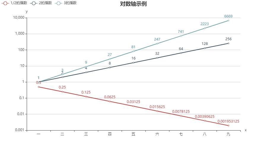
70.6 Line - Stacked_line_chart
import pyecharts.options as opts
from pyecharts.charts import Line

"""
Gallery 使用 pyecharts 1.1.0
参考地址: https://echarts.apache.org/examples/editor.html?c=line-stack

目前无法实现的功能:

暂无
"""


x_data = ["周一", "周二", "周三", "周四", "周五", "周六", "周日"]
y_data = [820, 932, 901, 934, 1290, 1330, 1320]


(
    Line()
    .add_xaxis(xaxis_data=x_data)
    .add_yaxis(
        series_name="邮件营销",
        stack="总量",
        y_axis=[120, 132, 101, 134, 90, 230, 210],
        label_opts=opts.LabelOpts(is_show=False),
    )
    .add_yaxis(
        series_name="联盟广告",
        stack="总量",
        y_axis=[220, 182, 191, 234, 290, 330, 310],
        label_opts=opts.LabelOpts(is_show=False),
    )
    .add_yaxis(
        series_name="视频广告",
        stack="总量",
        y_axis=[150, 232, 201, 154, 190, 330, 410],
        label_opts=opts.LabelOpts(is_show=False),
    )
    .add_yaxis(
        series_name="直接访问",
        stack="总量",
        y_axis=[320, 332, 301, 334, 390, 330, 320],
        label_opts=opts.LabelOpts(is_show=False),
    )
    .add_yaxis(
        series_name="搜索引擎",
        stack="总量",
        y_axis=[820, 932, 901, 934, 1290, 1330, 1320],
        label_opts=opts.LabelOpts(is_show=False),
    )
    .set_global_opts(
        title_opts=opts.TitleOpts(title="折线图堆叠"),
        tooltip_opts=opts.TooltipOpts(trigger="axis"),
        yaxis_opts=opts.AxisOpts(
            type_="value",
            axistick_opts=opts.AxisTickOpts(is_show=True),
            splitline_opts=opts.SplitLineOpts(is_show=True),
        ),
        xaxis_opts=opts.AxisOpts(type_="category", boundary_gap=False),
    )
    .render("stacked_line_chart.html")
)
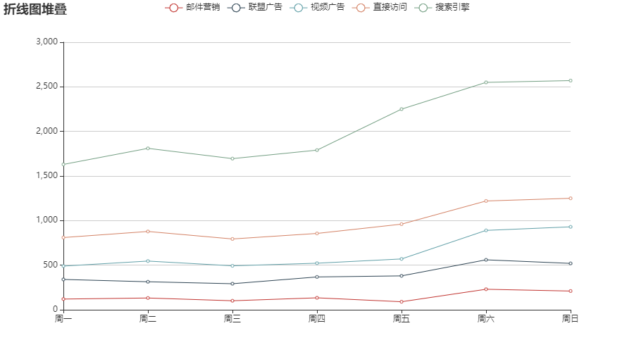
70.7 Line - Line_base
import pyecharts.options as opts
from pyecharts.charts import Line
from pyecharts.faker import Faker

c = (
    Line()
    .add_xaxis(Faker.choose())
    .add_yaxis("商家A", Faker.values())
    .add_yaxis("商家B", Faker.values())
    .set_global_opts(title_opts=opts.TitleOpts(title="Line-基本示例"))
    .render("line_base.html")
)
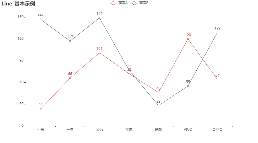
70.8 Line - Line_yaxis_log
import pyecharts.options as opts
from pyecharts.charts import Line

c = (
    Line()
    .add_xaxis(xaxis_data=["一", "二", "三", "四", "五", "六", "七", "八", "九"])
    .add_yaxis(
        "2 的指数",
        y_axis=[1, 2, 4, 8, 16, 32, 64, 128, 256],
        linestyle_opts=opts.LineStyleOpts(width=2),
    )
    .add_yaxis(
        "3 的指数",
        y_axis=[1, 3, 9, 27, 81, 247, 741, 2223, 6669],
        linestyle_opts=opts.LineStyleOpts(width=2),
    )
    .set_global_opts(
        title_opts=opts.TitleOpts(title="Line-对数轴示例"),
        xaxis_opts=opts.AxisOpts(name="x"),
        yaxis_opts=opts.AxisOpts(
            type_="log",
            name="y",
            splitline_opts=opts.SplitLineOpts(is_show=True),
            is_scale=True,
        ),
    )
    .render("line_yaxis_log.html")
)
?70.9 Line - Rainfall_and_water_flow
链接
代码过于复杂,略
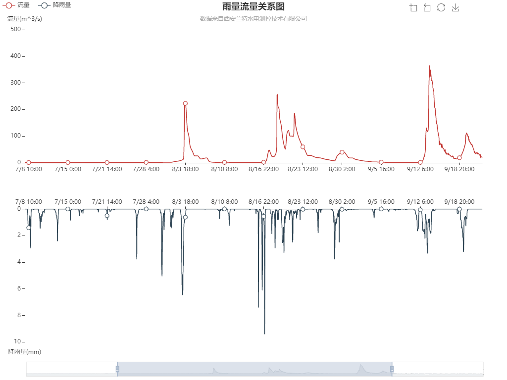
70.10 Line - Basic_area_chart
import pyecharts.options as opts
from pyecharts.charts import Line

"""
Gallery 使用 pyecharts 1.1.0
参考地址: https://echarts.apache.org/examples/editor.html?c=area-basic

目前无法实现的功能:

暂无
"""

x_data = ["Mon", "Tue", "Wed", "Thu", "Fri", "Sat", "Sun"]
y_data = [820, 932, 901, 934, 1290, 1330, 1320]


(
    Line()
    .add_xaxis(xaxis_data=x_data)
    .add_yaxis(
        series_name="",
        y_axis=y_data,
        symbol="emptyCircle",
        is_symbol_show=True,
        label_opts=opts.LabelOpts(is_show=False),
        areastyle_opts=opts.AreaStyleOpts(opacity=1, color="#C67570"),
    )
    .set_global_opts(
        tooltip_opts=opts.TooltipOpts(is_show=False),
        yaxis_opts=opts.AxisOpts(
            type_="value",
            axistick_opts=opts.AxisTickOpts(is_show=True),
            splitline_opts=opts.SplitLineOpts(is_show=True),
        ),
        xaxis_opts=opts.AxisOpts(type_="category", boundary_gap=False),
    )
    # 设置 boundary_gap 的时候一定要放在最后一个配置项里, 不然会被覆盖
    .render("basic_area_chart.html")
)
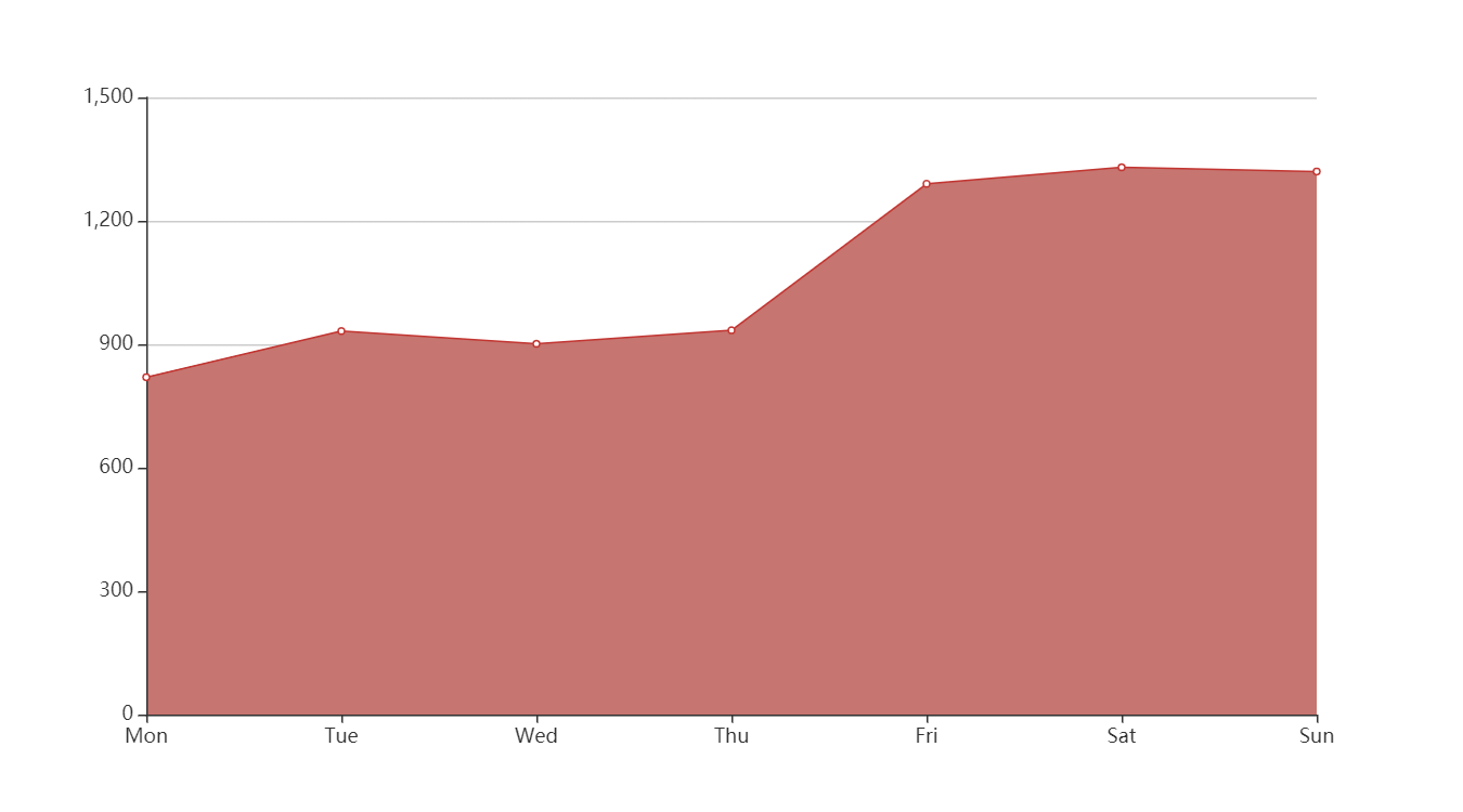
70.12 Line - Line_smooth
import pyecharts.options as opts
from pyecharts.charts import Line
from pyecharts.faker import Faker

c = (
    Line()
    .add_xaxis(Faker.choose())
    .add_yaxis("商家A", Faker.values(), is_smooth=True)
    .add_yaxis("商家B", Faker.values(), is_smooth=True)
    .set_global_opts(title_opts=opts.TitleOpts(title="Line-smooth"))
    .render("line_smooth.html")
)
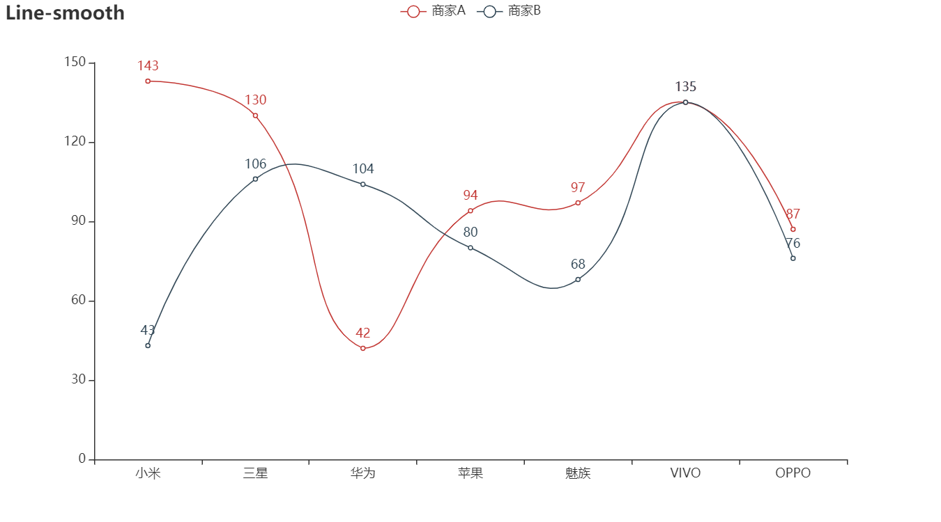
?70.13 Line - Multiple_x_axes
import pyecharts.options as opts
from pyecharts.charts import Line

# 将在 v1.1.0 中更改
from pyecharts.commons.utils import JsCode

"""
Gallery 使用 pyecharts 1.0.0
参考地址: https://echarts.apache.org/examples/editor.html?c=multiple-x-axis

目前无法实现的功能:

1、暂无
"""

js_formatter = """function (params) {
        console.log(params);
        return '降水量  ' + params.value + (params.seriesData.length ? ':' + params.seriesData[0].data : '');
    }"""

(
    Line(init_opts=opts.InitOpts(width="1600px", height="800px"))
    .add_xaxis(
        xaxis_data=[
            "2016-1",
            "2016-2",
            "2016-3",
            "2016-4",
            "2016-5",
            "2016-6",
            "2016-7",
            "2016-8",
            "2016-9",
            "2016-10",
            "2016-11",
            "2016-12",
        ]
    )
    .extend_axis(
        xaxis_data=[
            "2015-1",
            "2015-2",
            "2015-3",
            "2015-4",
            "2015-5",
            "2015-6",
            "2015-7",
            "2015-8",
            "2015-9",
            "2015-10",
            "2015-11",
            "2015-12",
        ],
        xaxis=opts.AxisOpts(
            type_="category",
            axistick_opts=opts.AxisTickOpts(is_align_with_label=True),
            axisline_opts=opts.AxisLineOpts(
                is_on_zero=False, linestyle_opts=opts.LineStyleOpts(color="#6e9ef1")
            ),
            axispointer_opts=opts.AxisPointerOpts(
                is_show=True, label=opts.LabelOpts(formatter=JsCode(js_formatter))
            ),
        ),
    )
    .add_yaxis(
        series_name="2015 降水量",
        is_smooth=True,
        symbol="emptyCircle",
        is_symbol_show=False,
        # xaxis_index=1,
        color="#d14a61",
        y_axis=[2.6, 5.9, 9.0, 26.4, 28.7, 70.7, 175.6, 182.2, 48.7, 18.8, 6.0, 2.3],
        label_opts=opts.LabelOpts(is_show=False),
        linestyle_opts=opts.LineStyleOpts(width=2),
    )
    .add_yaxis(
        series_name="2016 降水量",
        is_smooth=True,
        symbol="emptyCircle",
        is_symbol_show=False,
        color="#6e9ef1",
        y_axis=[3.9, 5.9, 11.1, 18.7, 48.3, 69.2, 231.6, 46.6, 55.4, 18.4, 10.3, 0.7],
        label_opts=opts.LabelOpts(is_show=False),
        linestyle_opts=opts.LineStyleOpts(width=2),
    )
    .set_global_opts(
        legend_opts=opts.LegendOpts(),
        tooltip_opts=opts.TooltipOpts(trigger="none", axis_pointer_type="cross"),
        xaxis_opts=opts.AxisOpts(
            type_="category",
            axistick_opts=opts.AxisTickOpts(is_align_with_label=True),
            axisline_opts=opts.AxisLineOpts(
                is_on_zero=False, linestyle_opts=opts.LineStyleOpts(color="#d14a61")
            ),
            axispointer_opts=opts.AxisPointerOpts(
                is_show=True, label=opts.LabelOpts(formatter=JsCode(js_formatter))
            ),
        ),
        yaxis_opts=opts.AxisOpts(
            type_="value",
            splitline_opts=opts.SplitLineOpts(
                is_show=True, linestyle_opts=opts.LineStyleOpts(opacity=1)
            ),
        ),
    )
    .render("multiple_x_axes.html")
)
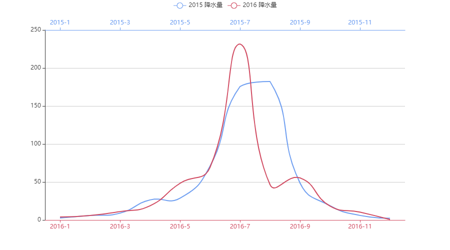
70.14 Line - Stacked_area_chart
import pyecharts.options as opts
from pyecharts.charts import Line

"""
Gallery 使用 pyecharts 1.1.0
参考地址: https://echarts.apache.org/examples/editor.html?c=area-stack

目前无法实现的功能:

暂无
"""


x_data = ["周一", "周二", "周三", "周四", "周五", "周六", "周日"]
y_data = [820, 932, 901, 934, 1290, 1330, 1320]


(
    Line()
    .add_xaxis(xaxis_data=x_data)
    .add_yaxis(
        series_name="邮件营销",
        stack="总量",
        y_axis=[120, 132, 101, 134, 90, 230, 210],
        areastyle_opts=opts.AreaStyleOpts(opacity=0.5),
        label_opts=opts.LabelOpts(is_show=False),
    )
    .add_yaxis(
        series_name="联盟广告",
        stack="总量",
        y_axis=[220, 182, 191, 234, 290, 330, 310],
        areastyle_opts=opts.AreaStyleOpts(opacity=0.5),
        label_opts=opts.LabelOpts(is_show=False),
    )
    .add_yaxis(
        series_name="视频广告",
        stack="总量",
        y_axis=[150, 232, 201, 154, 190, 330, 410],
        areastyle_opts=opts.AreaStyleOpts(opacity=0.5),
        label_opts=opts.LabelOpts(is_show=False),
    )
    .add_yaxis(
        series_name="直接访问",
        stack="总量",
        y_axis=[320, 332, 301, 334, 390, 330, 320],
        areastyle_opts=opts.AreaStyleOpts(opacity=0.5),
        label_opts=opts.LabelOpts(is_show=False),
    )
    .add_yaxis(
        series_name="搜索引擎",
        stack="总量",
        y_axis=[820, 932, 901, 934, 1290, 1330, 1320],
        areastyle_opts=opts.AreaStyleOpts(opacity=0.5),
        label_opts=opts.LabelOpts(is_show=True, position="top"),
    )
    .set_global_opts(
        title_opts=opts.TitleOpts(title="堆叠区域图"),
        tooltip_opts=opts.TooltipOpts(trigger="axis", axis_pointer_type="cross"),
        yaxis_opts=opts.AxisOpts(
            type_="value",
            axistick_opts=opts.AxisTickOpts(is_show=True),
            splitline_opts=opts.SplitLineOpts(is_show=True),
        ),
        xaxis_opts=opts.AxisOpts(type_="category", boundary_gap=False),
    )
    .render("stacked_area_chart.html")
)
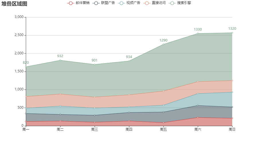
70.15 Line - Line_step
import pyecharts.options as opts
from pyecharts.charts import Line
from pyecharts.faker import Faker

c = (
    Line()
    .add_xaxis(Faker.choose())
    .add_yaxis("商家A", Faker.values(), is_step=True)
    .set_global_opts(title_opts=opts.TitleOpts(title="Line-阶梯图"))
    .render("line_step.html")
)
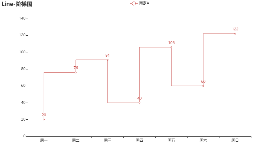
?70.16 Line - Line_color_with_js_func
import pyecharts.options as opts
from pyecharts.charts import Line
from pyecharts.commons.utils import JsCode


x_data = ["14", "15", "16", "17", "18", "19", "20", "21", "22", "23"]
y_data = [393, 438, 485, 631, 689, 824, 987, 1000, 1100, 1200]

background_color_js = (
    "new echarts.graphic.LinearGradient(0, 0, 0, 1, "
    "[{offset: 0, color: '#c86589'}, {offset: 1, color: '#06a7ff'}], false)"
)
area_color_js = (
    "new echarts.graphic.LinearGradient(0, 0, 0, 1, "
    "[{offset: 0, color: '#eb64fb'}, {offset: 1, color: '#3fbbff0d'}], false)"
)

c = (
    Line(init_opts=opts.InitOpts(bg_color=JsCode(background_color_js)))
    .add_xaxis(xaxis_data=x_data)
    .add_yaxis(
        series_name="注册总量",
        y_axis=y_data,
        is_smooth=True,
        is_symbol_show=True,
        symbol="circle",
        symbol_size=6,
        linestyle_opts=opts.LineStyleOpts(color="#fff"),
        label_opts=opts.LabelOpts(is_show=True, position="top", color="white"),
        itemstyle_opts=opts.ItemStyleOpts(
            color="red", border_color="#fff", border_width=3
        ),
        tooltip_opts=opts.TooltipOpts(is_show=False),
        areastyle_opts=opts.AreaStyleOpts(color=JsCode(area_color_js), opacity=1),
    )
    .set_global_opts(
        title_opts=opts.TitleOpts(
            title="OCTOBER 2015",
            pos_bottom="5%",
            pos_left="center",
            title_textstyle_opts=opts.TextStyleOpts(color="#fff", font_size=16),
        ),
        xaxis_opts=opts.AxisOpts(
            type_="category",
            boundary_gap=False,
            axislabel_opts=opts.LabelOpts(margin=30, color="#ffffff63"),
            axisline_opts=opts.AxisLineOpts(is_show=False),
            axistick_opts=opts.AxisTickOpts(
                is_show=True,
                length=25,
                linestyle_opts=opts.LineStyleOpts(color="#ffffff1f"),
            ),
            splitline_opts=opts.SplitLineOpts(
                is_show=True, linestyle_opts=opts.LineStyleOpts(color="#ffffff1f")
            ),
        ),
        yaxis_opts=opts.AxisOpts(
            type_="value",
            position="right",
            axislabel_opts=opts.LabelOpts(margin=20, color="#ffffff63"),
            axisline_opts=opts.AxisLineOpts(
                linestyle_opts=opts.LineStyleOpts(width=2, color="#fff")
            ),
            axistick_opts=opts.AxisTickOpts(
                is_show=True,
                length=15,
                linestyle_opts=opts.LineStyleOpts(color="#ffffff1f"),
            ),
            splitline_opts=opts.SplitLineOpts(
                is_show=True, linestyle_opts=opts.LineStyleOpts(color="#ffffff1f")
            ),
        ),
        legend_opts=opts.LegendOpts(is_show=False),
    )
    .render("line_color_with_js_func.html")
)
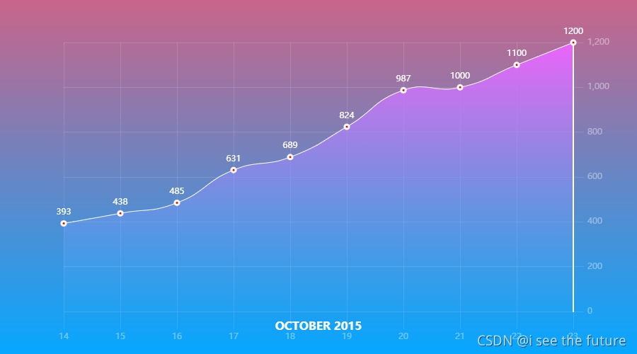
70.17 Line - Smoothed_line_chart
import pyecharts.options as opts
from pyecharts.charts import Line

"""
Gallery 使用 pyecharts 1.1.0
参考地址: https://echarts.apache.org/examples/editor.html?c=line-smooth

目前无法实现的功能:

暂无
"""


x_data = ["Mon", "Tue", "Wed", "Thu", "Fri", "Sat", "Sun"]
y_data = [820, 932, 901, 934, 1290, 1330, 1320]


(
    Line()
    .set_global_opts(
        tooltip_opts=opts.TooltipOpts(is_show=False),
        xaxis_opts=opts.AxisOpts(type_="category"),
        yaxis_opts=opts.AxisOpts(
            type_="value",
            axistick_opts=opts.AxisTickOpts(is_show=True),
            splitline_opts=opts.SplitLineOpts(is_show=True),
        ),
    )
    .add_xaxis(xaxis_data=x_data)
    .add_yaxis(
        series_name="",
        y_axis=y_data,
        symbol="emptyCircle",
        is_symbol_show=True,
        is_smooth=True,
        label_opts=opts.LabelOpts(is_show=False),
    )
    .render("smoothed_line_chart.html")
)
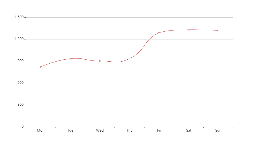
70.18 Line - Line_markpoint_custom
import pyecharts.options as opts
from pyecharts.charts import Line
from pyecharts.faker import Faker

x, y = Faker.choose(), Faker.values()
c = (
    Line()
    .add_xaxis(x)
    .add_yaxis(
        "商家A",
        y,
        markpoint_opts=opts.MarkPointOpts(
            data=[opts.MarkPointItem(name="自定义标记点", coord=[x[2], y[2]], value=y[2])]
        ),
    )
    .set_global_opts(title_opts=opts.TitleOpts(title="Line-MarkPoint(自定义)"))
    .render("line_markpoint_custom.html")
)
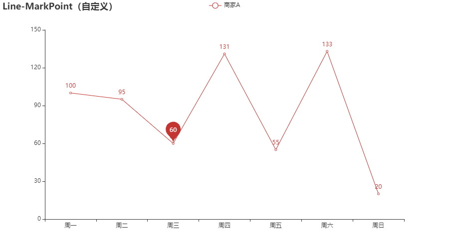
70.19 Line - Distribution_of_electricity
import pyecharts.options as opts
from pyecharts.charts import Line

"""
Gallery 使用 pyecharts 1.1.0
参考地址: https://www.echartsjs.com/examples/editor.html?c=line-sections

目前无法实现的功能:

1、visualMap 暂时无法设置隐藏
"""

x_data = [
    "00:00",
    "01:15",
    "02:30",
    "03:45",
    "05:00",
    "06:15",
    "07:30",
    "08:45",
    "10:00",
    "11:15",
    "12:30",
    "13:45",
    "15:00",
    "16:15",
    "17:30",
    "18:45",
    "20:00",
    "21:15",
    "22:30",
    "23:45",
]
y_data = [
    300,
    280,
    250,
    260,
    270,
    300,
    550,
    500,
    400,
    390,
    380,
    390,
    400,
    500,
    600,
    750,
    800,
    700,
    600,
    400,
]

(
    Line(init_opts=opts.InitOpts(width="1600px", height="800px"))
    .add_xaxis(xaxis_data=x_data)
    .add_yaxis(
        series_name="用电量",
        y_axis=y_data,
        is_smooth=True,
        label_opts=opts.LabelOpts(is_show=False),
        linestyle_opts=opts.LineStyleOpts(width=2),
    )
    .set_global_opts(
        title_opts=opts.TitleOpts(title="一天用电量分布", subtitle="纯属虚构"),
        tooltip_opts=opts.TooltipOpts(trigger="axis", axis_pointer_type="cross"),
        xaxis_opts=opts.AxisOpts(boundary_gap=False),
        yaxis_opts=opts.AxisOpts(
            axislabel_opts=opts.LabelOpts(formatter="{value} W"),
            splitline_opts=opts.SplitLineOpts(is_show=True),
        ),
        visualmap_opts=opts.VisualMapOpts(
            is_piecewise=True,
            dimension=0,
            pieces=[
                {"lte": 6, "color": "green"},
                {"gt": 6, "lte": 8, "color": "red"},
                {"gt": 8, "lte": 14, "color": "green"},
                {"gt": 14, "lte": 17, "color": "red"},
                {"gt": 17, "color": "green"},
            ],
        ),
    )
    .set_series_opts(
        markarea_opts=opts.MarkAreaOpts(
            data=[
                opts.MarkAreaItem(name="早高峰", x=("07:30", "10:00")),
                opts.MarkAreaItem(name="晚高峰", x=("17:30", "21:15")),
            ]
        )
    )
    .render("distribution_of_electricity.html")
)
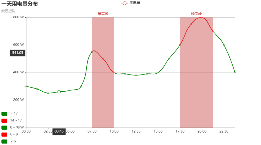
?70.20 Line - Beautiful_line_chart
import pyecharts.options as opts
from pyecharts.charts import Line, Grid
from pyecharts.commons.utils import JsCode

"""
参考地址: https://gallery.echartsjs.com/editor.html?c=xEyDk1hwBx
"""

x_data = ["14", "15", "16", "17", "18", "19", "20", "21", "22", "23"]
y_data = [393, 438, 485, 631, 689, 824, 987, 1000, 1100, 1200]

background_color_js = (
    "new echarts.graphic.LinearGradient(0, 0, 0, 1, "
    "[{offset: 0, color: '#c86589'}, {offset: 1, color: '#06a7ff'}], false)"
)
area_color_js = (
    "new echarts.graphic.LinearGradient(0, 0, 0, 1, "
    "[{offset: 0, color: '#eb64fb'}, {offset: 1, color: '#3fbbff0d'}], false)"
)

c = (
    Line(init_opts=opts.InitOpts(bg_color=JsCode(background_color_js)))
    .add_xaxis(xaxis_data=x_data)
    .add_yaxis(
        series_name="注册总量",
        y_axis=y_data,
        is_smooth=True,
        is_symbol_show=True,
        symbol="circle",
        symbol_size=6,
        linestyle_opts=opts.LineStyleOpts(color="#fff"),
        label_opts=opts.LabelOpts(is_show=True, position="top", color="white"),
        itemstyle_opts=opts.ItemStyleOpts(
            color="red", border_color="#fff", border_width=3
        ),
        tooltip_opts=opts.TooltipOpts(is_show=False),
        areastyle_opts=opts.AreaStyleOpts(color=JsCode(area_color_js), opacity=1),
    )
    .set_global_opts(
        title_opts=opts.TitleOpts(
            title="OCTOBER 2015",
            pos_bottom="5%",
            pos_left="center",
            title_textstyle_opts=opts.TextStyleOpts(color="#fff", font_size=16),
        ),
        xaxis_opts=opts.AxisOpts(
            type_="category",
            boundary_gap=False,
            axislabel_opts=opts.LabelOpts(margin=30, color="#ffffff63"),
            axisline_opts=opts.AxisLineOpts(is_show=False),
            axistick_opts=opts.AxisTickOpts(
                is_show=True,
                length=25,
                linestyle_opts=opts.LineStyleOpts(color="#ffffff1f"),
            ),
            splitline_opts=opts.SplitLineOpts(
                is_show=True, linestyle_opts=opts.LineStyleOpts(color="#ffffff1f")
            ),
        ),
        yaxis_opts=opts.AxisOpts(
            type_="value",
            position="right",
            axislabel_opts=opts.LabelOpts(margin=20, color="#ffffff63"),
            axisline_opts=opts.AxisLineOpts(
                linestyle_opts=opts.LineStyleOpts(width=2, color="#fff")
            ),
            axistick_opts=opts.AxisTickOpts(
                is_show=True,
                length=15,
                linestyle_opts=opts.LineStyleOpts(color="#ffffff1f"),
            ),
            splitline_opts=opts.SplitLineOpts(
                is_show=True, linestyle_opts=opts.LineStyleOpts(color="#ffffff1f")
            ),
        ),
        legend_opts=opts.LegendOpts(is_show=False),
    )
)

(
    Grid()
    .add(
        c,
        grid_opts=opts.GridOpts(
            pos_top="20%",
            pos_left="10%",
            pos_right="10%",
            pos_bottom="15%",
            is_contain_label=True,
        ),
    )
    .render("beautiful_line_chart.html")
)
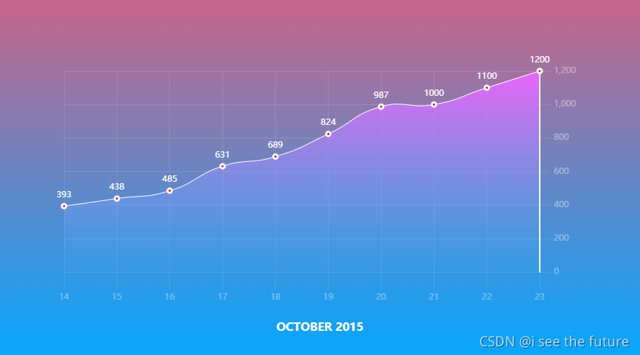
?70.21 Line - Beijing_aqi(难)
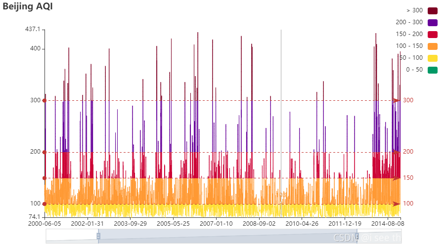
70.22 Line - Line_style_and_item_style
import pyecharts.options as opts
from pyecharts.charts import Line

"""
Gallery 使用 pyecharts 1.1.0
参考地址: https://www.echartsjs.com/examples/editor.html?c=line-style

目前无法实现的功能:

暂无
"""


(
    Line(init_opts=opts.InitOpts(width="1280px", height="720px"))
    .add_xaxis(xaxis_data=["Mon", "Tue", "Wed", "Thu", "Fri", "Sat", "Sun"])
    .add_yaxis(
        series_name="",
        y_axis=[120, 200, 150, 80, 70, 110, 130],
        symbol="triangle",
        symbol_size=20,
        linestyle_opts=opts.LineStyleOpts(color="green", width=4, type_="dashed"),
        label_opts=opts.LabelOpts(is_show=False),
        itemstyle_opts=opts.ItemStyleOpts(
            border_width=3, border_color="yellow", color="blue"
        ),
    )
    .set_global_opts(
        xaxis_opts=opts.AxisOpts(type_="category"),
        yaxis_opts=opts.AxisOpts(
            type_="value",
            axistick_opts=opts.AxisTickOpts(is_show=True),
            splitline_opts=opts.SplitLineOpts(is_show=True),
        ),
        tooltip_opts=opts.TooltipOpts(is_show=False),
    )
    .render("line_style_and_item_style.html")
)
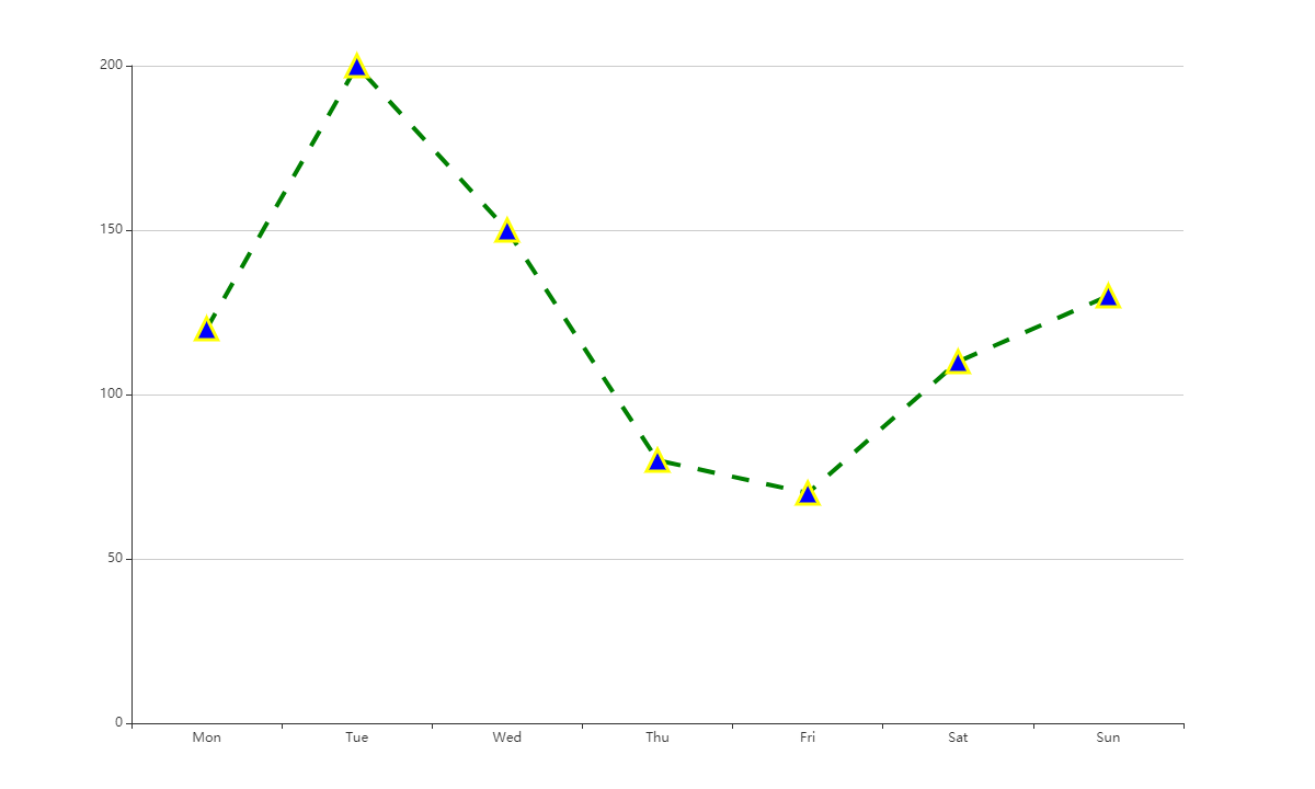
70.23 Line - Line_markpoint
import pyecharts.options as opts
from pyecharts.charts import Line
from pyecharts.faker import Faker

c = (
    Line()
    .add_xaxis(Faker.choose())
    .add_yaxis(
        "商家A",
        Faker.values(),
        markpoint_opts=opts.MarkPointOpts(data=[opts.MarkPointItem(type_="min")]),
    )
    .add_yaxis(
        "商家B",
        Faker.values(),
        markpoint_opts=opts.MarkPointOpts(data=[opts.MarkPointItem(type_="max")]),
    )
    .set_global_opts(title_opts=opts.TitleOpts(title="Line-MarkPoint"))
    .render("line_markpoint.html")
)

70.24 Line - Line_markline
import pyecharts.options as opts
from pyecharts.charts import Line
from pyecharts.faker import Faker

c = (
    Line()
    .add_xaxis(Faker.choose())
    .add_yaxis(
        "商家A",
        Faker.values(),
        markline_opts=opts.MarkLineOpts(data=[opts.MarkLineItem(type_="average")]),
    )
    .add_yaxis(
        "商家B",
        Faker.values(),
        markline_opts=opts.MarkLineOpts(data=[opts.MarkLineItem(type_="average")]),
    )
    .set_global_opts(title_opts=opts.TitleOpts(title="Line-MarkLine"))
    .render("line_markline.html")
)
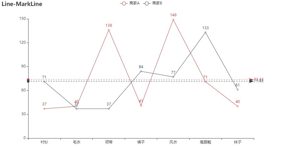
70.25 Line - Line_itemstyle
import pyecharts.options as opts
from pyecharts.charts import Line
from pyecharts.faker import Faker

c = (
    Line()
    .add_xaxis(xaxis_data=Faker.choose())
    .add_yaxis(
        "商家A",
        Faker.values(),
        symbol="triangle",
        symbol_size=20,
        linestyle_opts=opts.LineStyleOpts(color="green", width=4, type_="dashed"),
        itemstyle_opts=opts.ItemStyleOpts(
            border_width=3, border_color="yellow", color="blue"
        ),
    )
    .set_global_opts(title_opts=opts.TitleOpts(title="Line-ItemStyle"))
    .render("line_itemstyle.html")
)
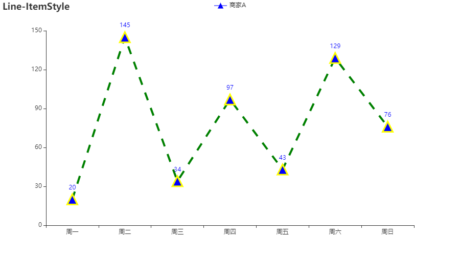
70.26 Line - Line_area_style
import pyecharts.options as opts
from pyecharts.charts import Line
from pyecharts.faker import Faker

c = (
    Line()
    .add_xaxis(Faker.choose())
    .add_yaxis("商家A", Faker.values(), areastyle_opts=opts.AreaStyleOpts(opacity=0.5))
    .add_yaxis("商家B", Faker.values(), areastyle_opts=opts.AreaStyleOpts(opacity=0.5))
    .set_global_opts(title_opts=opts.TitleOpts(title="Line-面积图"))
    .render("line_area_style.html")
)
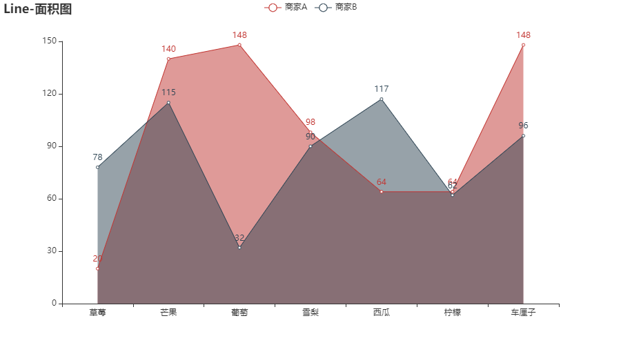
70.27 Season实践:Line运用pieces设定不同时期的颜色
自定义的每一段的范围,以及每一段的文字,以及每一段的特别的样式。
    # 自定义的每一段的范围,以及每一段的文字,以及每一段的特别的样式。例如:
    # pieces: [
    #   {"min": 1500}, // 不指定 max,表示 max 为无限大(Infinity)。
    #   {"min": 900, "max": 1500},
    #   {"min": 310, "max": 1000},
    #   {"min": 200, "max": 300},
    #   {"min": 10, "max": 200, "label": '10 到 200(自定义label)'},
    #   {"value": 123, "label": '123(自定义特殊颜色)', "color": 'grey'}, //表示 value 等于 123 的情况
    #   {"max": 5}     // 不指定 min,表示 min 为无限大(-Infinity)。
    # ]
    pieces: Optional[Sequence] = None,
            visualmap_opts=opts.VisualMapOpts(
                is_piecewise=True,
                dimension=0,
                pieces=[
                    {"lte": 6, "color": "green"},
                    {"gt": 6, "lte": 8, "color": "red"},
                    {"gt": 8, "lte": 14, "color": "green"},
                    {"gt": 14, "lte": 17, "color": "red"},
                    {"gt": 17, "color": "green"},
                ],
            ),
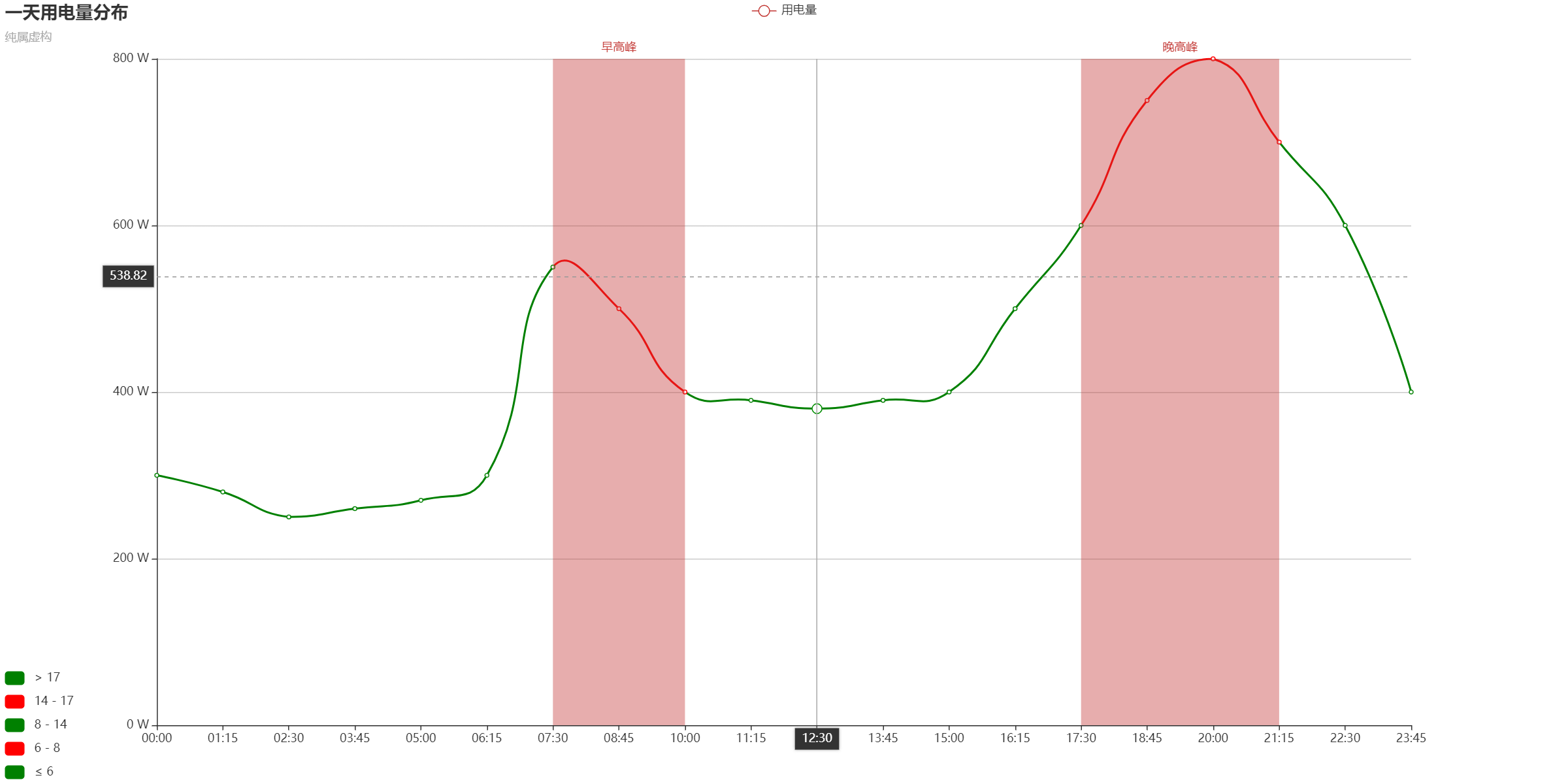
- 完整代码
def Distribution_of_electricity():
    x_data = ["00:00","01:15","02:30","03:45","05:00", "06:15","07:30","08:45","10:00","11:15","12:30","13:45","15:00","16:15","17:30","18:45","20:00","21:15","22:30","23:45",]
    y_data = [300,280,250,260,270,300,550,500,400,390,380,390,400,500,600,750,800,700,600,400,]

    c = (
        Line(init_opts=opts.InitOpts(width="1600px", height="800px"))
        .add_xaxis(xaxis_data=x_data)
        .add_yaxis(
            series_name="用电量",
            y_axis=y_data,
            is_smooth=True,
            label_opts=opts.LabelOpts(is_show=False),
            linestyle_opts=opts.LineStyleOpts(width=2),
        )
        .set_global_opts(
            title_opts=opts.TitleOpts(title="一天用电量分布", subtitle="纯属虚构"),
            tooltip_opts=opts.TooltipOpts(trigger="axis", axis_pointer_type="cross"),
            xaxis_opts=opts.AxisOpts(boundary_gap=False),
            yaxis_opts=opts.AxisOpts(
                axislabel_opts=opts.LabelOpts(formatter="{value} W"),
                splitline_opts=opts.SplitLineOpts(is_show=True),
            ),
            visualmap_opts=opts.VisualMapOpts(
                is_piecewise=True,
                dimension=0,
                pieces=[
                    {"lte": 6, "color": "green"},
                    {"gt": 6, "lte": 8, "color": "red"},
                    {"gt": 8, "lte": 14, "color": "green"},
                    {"gt": 14, "lte": 17, "color": "red"},
                    {"gt": 17, "color": "green"},
                ],
            ),
        )
        .set_series_opts(
            markarea_opts=opts.MarkAreaOpts(
                data=[
                    opts.MarkAreaItem(name="早高峰", x=("07:30", "10:00")),
                    opts.MarkAreaItem(name="晚高峰", x=("17:30", "21:15")),
                ]
            )
        )
        #.render("distribution_of_electricity.html")
    )
    return c
71.PictorialBar:象形柱状图
- class pyecharts.charts.PictorialBar(RectChart)
class PictorialBar(
    # 初始化配置项,参考 `global_options.InitOpts`
    init_opts: opts.InitOpts = opts.InitOpts()
)
- func pyecharts.charts.PictorialBar.add_yaxis
def add_yaxis(
    # 系列名称,用于 tooltip 的显示,legend 的图例筛选。
    series_name: str,

    # 系列数据
    y_axis: Sequence,

    # 图形类型。
    # ECharts 提供的标记类型包括 'circle', 'rect', 'roundRect', 'triangle',
    # 'diamond', 'pin', 'arrow', 'none'
    # 可以通过 'image://url' 设置为图片,其中 URL 为图片的链接,或者 dataURI。
    # URL 为图片链接例如:'image://http://xxx.xxx.xxx/a/b.png'
    # URL 为 dataURI 例如:'image://data:image/gif;base64,R0lGODlhEAAQAMQAAORHHOVSKudfO...
    # 可以通过 'path://' 将图标设置为任意的矢量路径。这种方式相比于使用图片的方式,不用担心因为缩放而产生锯齿或模糊,
    # 而且可以设置为任意颜色。路径图形会自适应调整为合适的大小。路径的格式参见 SVG PathData。
    # 可以从 Adobe Illustrator 等工具编辑导出。例如:
    # 'path://M30.9,53.2C16.8,53.2,5.3,41.7,5.3,27.6S16.8,2,30.9,2C45,2,56.4,13.5,56.4,2...'
    symbol: Optional[str] = None,

    # 图形的大小。
    # 可以用数组分开表示宽和高,例如 [20, 10] 表示标记宽为20,
    # 高为 10,也可以设置成诸如 10 这样单一的数字,表示 [10, 10]。
    # 可以设置成绝对值(如 10),也可以设置成百分比(如 '120%'、['55%', 23])。
    symbol_size: Union[Numeric, Sequence, None] = None,

    # 图形的定位位置。可取值:
    # 'start':图形边缘与柱子开始的地方内切。
    # 'end':图形边缘与柱子结束的地方内切。
    # 'center':图形在柱子里居中。
    symbol_pos: Optional[str] = None,

    # 图形相对于原本位置的偏移。symbolOffset 是图形定位中最后计算的一个步骤,
    # 可以对图形计算出来的位置进行微调。
    # 可以设置成绝对值(如 10),也可以设置成百分比(如 '120%'、['55%', 23])。
    # 当设置为百分比时,表示相对于自身尺寸 symbolSize 的百分比。
    # 例如 [0, '-50%'] 就是把图形向上移动了自身尺寸的一半的位置。
    symbol_offset: Optional[Sequence] = None,

    # 图形的旋转角度。
    # 注意,symbolRotate 并不会影响图形的定位(哪怕超出基准柱的边界),而只是单纯得绕自身中心旋转。
    # 此属性可以被设置在系列的 根部,表示对此系列中所有数据都生效;
    # 也可以被设置在 data 中的 每个数据项中,表示只对此数据项生效。
    symbol_rotate: Optional[Numeric] = None,

    # 指定图形元素是否重复。值可为:
    # false/null/undefined:不重复,即每个数据值用一个图形元素表示。
    # true:使图形元素重复,即每个数据值用一组重复的图形元素表示。重复的次数依据 data 计算得到。
    # a number:使图形元素重复,即每个数据值用一组重复的图形元素表示。重复的次数是给定的定值。
    # 'fixed':使图形元素重复,即每个数据值用一组重复的图形元素表示。
    # 重复的次数依据 symbolBoundingData 计算得到,即与 data 无关。这在此图形被用于做背景时有用。
    symbol_repeat: Optional[str] = None,

    # 指定图形元素重复时,绘制的顺序。这个属性在两种情况下有用处:
    # 当 symbolMargin 设置为负值时,重复的图形会互相覆盖,这是可以使用 symbolRepeatDirection 来指定覆盖顺序。
    # 当 animationDelay 或 animationDelayUpdate 被使用时,symbolRepeatDirection 指定了 index 顺序。
    # 这个属性的值可以是:'start' 或 'end'。
    symbol_repeat_direction: Optional[str] = None,

    # 图形的两边间隔(『两边』是指其数值轴方向的两边)。可以是绝对数值(如 20),或者百分比值(如 '-30%'),
    # 表示相对于自身尺寸 symbolSize 的百分比。只有当 symbolRepeat 被使用时有意义。
    # 可以是正值,表示间隔大;也可以是负数。当 symbolRepeat 被使用时,负数时能使图形重叠。
    # 可以在其值结尾处加一个 "!",如 "30%!" 或 25!,表示第一个图形的开始和最后一个图形结尾留白,
    # 不紧贴边界。默认会紧贴边界。
    symbol_margin: Union[Numeric, str, None] = None,

    # 是否剪裁图形。
    # false/null/undefined:图形本身表示数值大小。
    # true:图形被剪裁后剩余的部分表示数值大小。
    # symbolClip 常在这种场景下使用:同时表达『总值』和『当前数值』。在这种场景下,可以使用两个系列,
    # 一个系列是完整的图形,当做『背景』来表达总数值,另一个系列是使用 symbolClip 进行剪裁过的图形,表达当前数值。
    is_symbol_clip: bool = False,

    # 是否选中图例
    is_selected: bool = True,

    # 使用的 x 轴的 index,在单个图表实例中存在多个 x 轴的时候有用。
    xaxis_index: Optional[Numeric] = None,

    # 使用的 y 轴的 index,在单个图表实例中存在多个 y 轴的时候有用。
    yaxis_index: Optional[Numeric] = None,

    # 系列 label 颜色
    color: Optional[str] = None,

    # 同一系列的柱间距离,默认为类目间距的 20%,可设固定值
    category_gap: Union[Numeric, str] = "20%",

    # 不同系列的柱间距离,为百分比(如 '30%',表示柱子宽度的 30%)。
    # 如果想要两个系列的柱子重叠,可以设置 gap 为 '-100%'。这在用柱子做背景的时候有用。
    gap: Optional[str] = None,

    # 标签配置项,参考 `series_options.LabelOpts`
    label_opts: Union[opts.LabelOpts, dict] = opts.LabelOpts(),

    # 标记点配置项,参考 `series_options.MarkPointOpts`
    markpoint_opts: Union[opts.MarkPointOpts, dict, None] = None,

    # 标记线配置项,参考 `series_options.MarkLineOpts`
    markline_opts: Union[opts.MarkLineOpts, dict, None] = None,

    # 提示框组件配置项,参考 `series_options.TooltipOpts`
    tooltip_opts: Union[opts.TooltipOpts, dict, None] = None,

    # 图元样式配置项,参考 `series_options.ItemStyleOpts`
    itemstyle_opts: Union[opts.ItemStyleOpts, dict, None] = None,

    # 可以定义 data 的哪个维度被编码成什么。
    encode: types.Union[types.JsCode, dict] = None,
)
71.1 Pictorialbar - Pictorialbar_base
from pyecharts import options as opts
from pyecharts.charts import PictorialBar
from pyecharts.globals import SymbolType

location = ["山西", "四川", "西藏", "北京", "上海", "内蒙古", "云南", "黑龙江", "广东", "福建"]
values = [13, 42, 67, 81, 86, 94, 166, 220, 249, 262]

c = (
    PictorialBar()
    .add_xaxis(location)
    .add_yaxis(
        "",
        values,
        label_opts=opts.LabelOpts(is_show=False),
        symbol_size=18,
        symbol_repeat="fixed",
        symbol_offset=[0, 0],
        is_symbol_clip=True,
        symbol=SymbolType.ROUND_RECT,
    )
    .reversal_axis()
    .set_global_opts(
        title_opts=opts.TitleOpts(title="PictorialBar-各省份人口数量(虚假数据)"),
        xaxis_opts=opts.AxisOpts(is_show=False),
        yaxis_opts=opts.AxisOpts(
            axistick_opts=opts.AxisTickOpts(is_show=False),
            axisline_opts=opts.AxisLineOpts(
                linestyle_opts=opts.LineStyleOpts(opacity=0)
            ),
        ),
    )
    .render("pictorialbar_base.html")
)
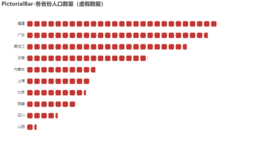
71.2 Pictorialbar - Pictorialbar_multi_custom_symbols
import json

from pyecharts import options as opts
from pyecharts.charts import PictorialBar

location = ["山西", "四川", "西藏", "北京", "上海", "内蒙古", "云南", "黑龙江", "广东", "福建"]
values = [13, 42, 67, 81, 86, 94, 166, 220, 249, 262]


with open("symbol.json", "r", encoding="utf-8") as f:
    symbols = json.load(f)

c = (
    PictorialBar()
    .add_xaxis(["reindeer", "ship", "plane", "train", "car"])
    .add_yaxis(
        "2015",
        [
            {"value": 157, "symbol": symbols["reindeer"]},
            {"value": 21, "symbol": symbols["ship"]},
            {"value": 66, "symbol": symbols["plane"]},
            {"value": 78, "symbol": symbols["train"]},
            {"value": 123, "symbol": symbols["car"]},
        ],
        label_opts=opts.LabelOpts(is_show=False),
        symbol_size=22,
        symbol_repeat="fixed",
        symbol_offset=[0, 5],
        is_symbol_clip=True,
    )
    .add_yaxis(
        "2016",
        [
            {"value": 184, "symbol": symbols["reindeer"]},
            {"value": 29, "symbol": symbols["ship"]},
            {"value": 73, "symbol": symbols["plane"]},
            {"value": 91, "symbol": symbols["train"]},
            {"value": 95, "symbol": symbols["car"]},
        ],
        label_opts=opts.LabelOpts(is_show=False),
        symbol_size=22,
        symbol_repeat="fixed",
        symbol_offset=[0, -25],
        is_symbol_clip=True,
    )
    .reversal_axis()
    .set_global_opts(
        title_opts=opts.TitleOpts(title="PictorialBar-Vehicles in X City"),
        xaxis_opts=opts.AxisOpts(is_show=False),
        yaxis_opts=opts.AxisOpts(
            axistick_opts=opts.AxisTickOpts(is_show=False),
            axisline_opts=opts.AxisLineOpts(
                linestyle_opts=opts.LineStyleOpts(opacity=0)
            ),
        ),
    )
    .render("pictorialbar_multi_custom_symbols.html")
)

71.3 Pictorialbar - Pictorialbar_custom_symbol
import json

from pyecharts import options as opts
from pyecharts.charts import PictorialBar

location = ["山西", "四川", "西藏", "北京", "上海", "内蒙古", "云南", "黑龙江", "广东", "福建"]
values = [13, 42, 67, 81, 86, 94, 166, 220, 249, 262]


with open("symbol.json", "r", encoding="utf-8") as f:
    symbols = json.load(f)


c = (
    PictorialBar()
    .add_xaxis(location)
    .add_yaxis(
        "",
        values,
        label_opts=opts.LabelOpts(is_show=False),
        symbol_size=22,
        symbol_repeat="fixed",
        symbol_offset=[0, -5],
        is_symbol_clip=True,
        symbol=symbols["boy"],
    )
    .reversal_axis()
    .set_global_opts(
        title_opts=opts.TitleOpts(title="PictorialBar-自定义 Symbol"),
        xaxis_opts=opts.AxisOpts(is_show=False),
        yaxis_opts=opts.AxisOpts(
            axistick_opts=opts.AxisTickOpts(is_show=False),
            axisline_opts=opts.AxisLineOpts(
                linestyle_opts=opts.LineStyleOpts(opacity=0)
            ),
        ),
    )
    .render("pictorialbar_custom_symbol.html")
)

71.4 Season实践:PictorialBar-自定义图例
自定义图例可以是任意的图片
def Pictorialbar_custom_symbol():
    location = ["山西", "四川", "西藏", "北京", "上海", "内蒙古", "云南", "黑龙江", "广东", "福建"]
    values = [13, 42, 67, 81, 86, 94, 166, 220, 249, 262]

    c = (
        PictorialBar()
        .add_xaxis(location)
        .add_yaxis(
            "",
            values,
            label_opts=opts.LabelOpts(is_show=False),
            symbol_size=18,
            symbol_repeat="fixed",
            symbol_offset=[0, 0],
            is_symbol_clip=True,
            #symbol=SymbolType.ROUND_RECT,
            symbol = 'image://海星.png',
            color='green',
        )
        .reversal_axis()
        .set_global_opts(
            title_opts=opts.TitleOpts(title="PictorialBar-自定义 Symbol"),
            xaxis_opts=opts.AxisOpts(is_show=False),
            yaxis_opts=opts.AxisOpts(
                axistick_opts=opts.AxisTickOpts(is_show=False),
                axisline_opts=opts.AxisLineOpts(
                    linestyle_opts=opts.LineStyleOpts(opacity=0)
                ),
            ),
        )
        #.render("pictorialbar_base.html")
    )
    return c

71.5 Season实践:PictorialBar-自定义图例2
自定义图例可以是任意的图片
def Pictorialbar_multi_custom_symbols():
    location = ["山西", "四川", "西藏", "北京", "上海", "内蒙古", "云南", "黑龙江", "广东", "福建"]
    values = [13, 42, 67, 81, 86, 94, 166, 220, 249, 262]


    with open("symbol.json", "r", encoding="utf-8") as f:
        symbols = json.load(f)

    c = (
        PictorialBar()
        .add_xaxis(["reindeer", "ship", "plane", "train", "car"])
        .add_yaxis(
            "2015",
            [
                {"value": 157, "symbol": 'image://海星.png'},
                {"value": 21, "symbol": symbols["ship"]},
                {"value": 66, "symbol": symbols["plane"]},
                {"value": 78, "symbol": symbols["train"]},
                {"value": 123, "symbol": symbols["car"]},
            ],
            label_opts=opts.LabelOpts(is_show=False),
            symbol_size=22,
            symbol_repeat="fixed",
            symbol_offset=[0, 5],
            is_symbol_clip=True,
        )
        .add_yaxis(
            "2016",
            [
                {"value": 184, "symbol": 'image://海星.png'},
                {"value": 29, "symbol": symbols["ship"]},
                {"value": 73, "symbol": symbols["plane"]},
                {"value": 91, "symbol": symbols["train"]},
                {"value": 95, "symbol": symbols["car"]},
            ],
            label_opts=opts.LabelOpts(is_show=False),
            symbol_size=22,
            symbol_repeat="fixed",
            symbol_offset=[0, -25],
            is_symbol_clip=True,
        )
        .reversal_axis()
        .set_global_opts(
            title_opts=opts.TitleOpts(title="PictorialBar-Vehicles in X City"),
            xaxis_opts=opts.AxisOpts(is_show=False),
            yaxis_opts=opts.AxisOpts(
                axistick_opts=opts.AxisTickOpts(is_show=False),
                axisline_opts=opts.AxisLineOpts(
                    linestyle_opts=opts.LineStyleOpts(opacity=0)
                ),
            ),
        )
    #    .render("pictorialbar_multi_custom_symbols.html")
    )
    return c

72.Scatter:散点图
- class pyecharts.charts.Scatter(RectChart)
class Scatter(
    # 初始化配置项,参考 `global_options.InitOpts`
    init_opts: opts.InitOpts = opts.InitOpts()
)
- func pyecharts.charts.Scatter.add_yaxis
def add_yaxis(
    # 系列名称,用于 tooltip 的显示,legend 的图例筛选。
    series_name: str,

    # 系列数据
    y_axis: Sequence,

    # 是否选中图例
    is_selected: bool = True,

    # 使用的 x 轴的 index,在单个图表实例中存在多个 x 轴的时候有用。
    xaxis_index: Optional[Numeric] = None,

    # 使用的 y 轴的 index,在单个图表实例中存在多个 y 轴的时候有用。
    yaxis_index: Optional[Numeric] = None,

    # 系列 label 颜色
    color: Optional[str] = None,

    # 标记的图形。
    # ECharts 提供的标记类型包括 'circle', 'rect', 'roundRect', 'triangle',
    # 'diamond', 'pin', 'arrow', 'none'
    # 可以通过 'image://url' 设置为图片,其中 URL 为图片的链接,或者 dataURI。
    symbol: Optional[str] = None,

    # 标记的大小,可以设置成诸如 10 这样单一的数字,也可以用数组分开表示宽和高,
    # 例如 [20, 10] 表示标记宽为 20,高为 10。
    symbol_size: Numeric = 10,

    # 标记的旋转角度。注意在 markLine 中当 symbol 为 'arrow' 时会忽略 symbolRotate 强制设置为切线的角度。
    symbol_rotate: types.Optional[types.Numeric] = None,

    # 标签配置项,参考 `series_options.LabelOpts`
    label_opts: Union[opts.LabelOpts, dict] = opts.LabelOpts(position="right"),

    # 标记点配置项,参考 `series_options.MarkPointOpts`
    markpoint_opts: Union[opts.MarkPointOpts, dict, None] = None,

    # 标记线配置项,参考 `series_options.MarkLineOpts`
    markline_opts: Union[opts.MarkLineOpts, dict, None] = None,

    # 图表标域,常用于标记图表中某个范围的数据,参考 `series_options.MarkAreaOpts`
    markarea_opts: types.MarkArea = None,

    # 提示框组件配置项,参考 `series_options.TooltipOpts`
    tooltip_opts: Union[opts.TooltipOpts, dict, None] = None,

    # 图元样式配置项,参考 `series_options.ItemStyleOpts`
    itemstyle_opts: Union[opts.ItemStyleOpts, dict, None] = None,

    # 可以定义 data 的哪个维度被编码成什么。
    encode: types.Union[types.JSFunc, dict, None] = None,
)
- ScatterItem:散点图数据项
class ScatterItem(
    # 数据项名称。
    name: Union[str, Numeric] = None,

    # 数据项值。
    value: Union[str, Numeric] = None,

    # 单个数据标记的图形。
    # ECharts 提供的标记类型包括
    # 'circle', 'rect', 'roundRect', 'triangle', 'diamond', 'pin', 'arrow', 'none'
    # 可以通过 'image://url' 设置为图片,其中 URL 为图片的链接,或者 dataURI。
    # 可以通过 'path://' 将图标设置为任意的矢量路径。
    symbol: Optional[str] = None,

    # 单个数据标记的大小,可以设置成诸如 10 这样单一的数字
    # 也可以用数组分开表示宽和高,例如 [20, 10] 表示标记宽为20,高为10。
    symbol_size: Union[Sequence[Numeric], Numeric] = None,

    # 单个数据标记的旋转角度(而非弧度)。正
    symbol_rotate: Optional[Numeric] = None,

    # 如果 symbol 是 path:// 的形式,是否在缩放时保持该图形的长宽比。
    symbol_keep_aspect: bool = False,

    # 单个数据标记相对于原本位置的偏移。
    symbol_offset: Optional[Sequence] = None,

    # 标签配置项,参考 `series_options.LabelOpts`
    label_opts: Union[LabelOpts, dict, None] = None,

    # 图元样式配置项,参考 `series_options.ItemStyleOpts`
    itemstyle_opts: Union[ItemStyleOpts, dict, None] = None,

    # 提示框组件配置项,参考 `series_options.TooltipOpts`
    tooltip_opts: Union[TooltipOpts, dict, None] = None,
)
72.1 Scatter - Basic_scatter_chart
import pyecharts.options as opts
from pyecharts.charts import Scatter

"""
Gallery 使用 pyecharts 1.1.0
参考地址: https://echarts.apache.org/examples/editor.html?c=scatter-simple

目前无法实现的功能:

1、暂无
"""

data = [
    [10.0, 8.04],
    [8.0, 6.95],
    [13.0, 7.58],
    [9.0, 8.81],
    [11.0, 8.33],
    [14.0, 9.96],
    [6.0, 7.24],
    [4.0, 4.26],
    [12.0, 10.84],
    [7.0, 4.82],
    [5.0, 5.68],
]
data.sort(key=lambda x: x[0])
x_data = [d[0] for d in data]
y_data = [d[1] for d in data]

(
    Scatter(init_opts=opts.InitOpts(width="1600px", height="1000px"))
    .add_xaxis(xaxis_data=x_data)
    .add_yaxis(
        series_name="",
        y_axis=y_data,
        symbol_size=20,
        label_opts=opts.LabelOpts(is_show=False),
    )
    .set_series_opts()
    .set_global_opts(
        xaxis_opts=opts.AxisOpts(
            type_="value", splitline_opts=opts.SplitLineOpts(is_show=True)
        ),
        yaxis_opts=opts.AxisOpts(
            type_="value",
            axistick_opts=opts.AxisTickOpts(is_show=True),
            splitline_opts=opts.SplitLineOpts(is_show=True),
        ),
        tooltip_opts=opts.TooltipOpts(is_show=False),
    )
    .render("basic_scatter_chart.html")
)
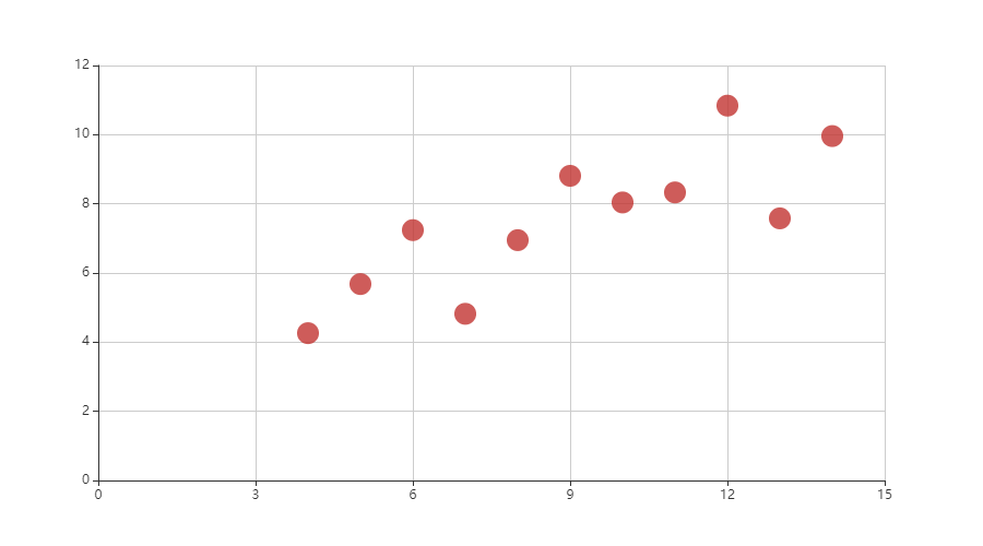
72.2 Scatter - Scatter_multi_dimension
from pyecharts import options as opts
from pyecharts.charts import Scatter
from pyecharts.commons.utils import JsCode
from pyecharts.faker import Faker

c = (
    Scatter()
    .add_xaxis(Faker.choose())
    .add_yaxis(
        "商家A",
        [list(z) for z in zip(Faker.values(), Faker.choose())],
        label_opts=opts.LabelOpts(
            formatter=JsCode(
                "function(params){return params.value[1] +' : '+ params.value[2];}"
            )
        ),
    )
    .set_global_opts(
        title_opts=opts.TitleOpts(title="Scatter-多维度数据"),
        tooltip_opts=opts.TooltipOpts(
            formatter=JsCode(
                "function (params) {return params.name + ' : ' + params.value[2];}"
            )
        ),
        visualmap_opts=opts.VisualMapOpts(
            type_="color", max_=150, min_=20, dimension=1
        ),
    )
    .render("scatter_multi_dimension.html")
)
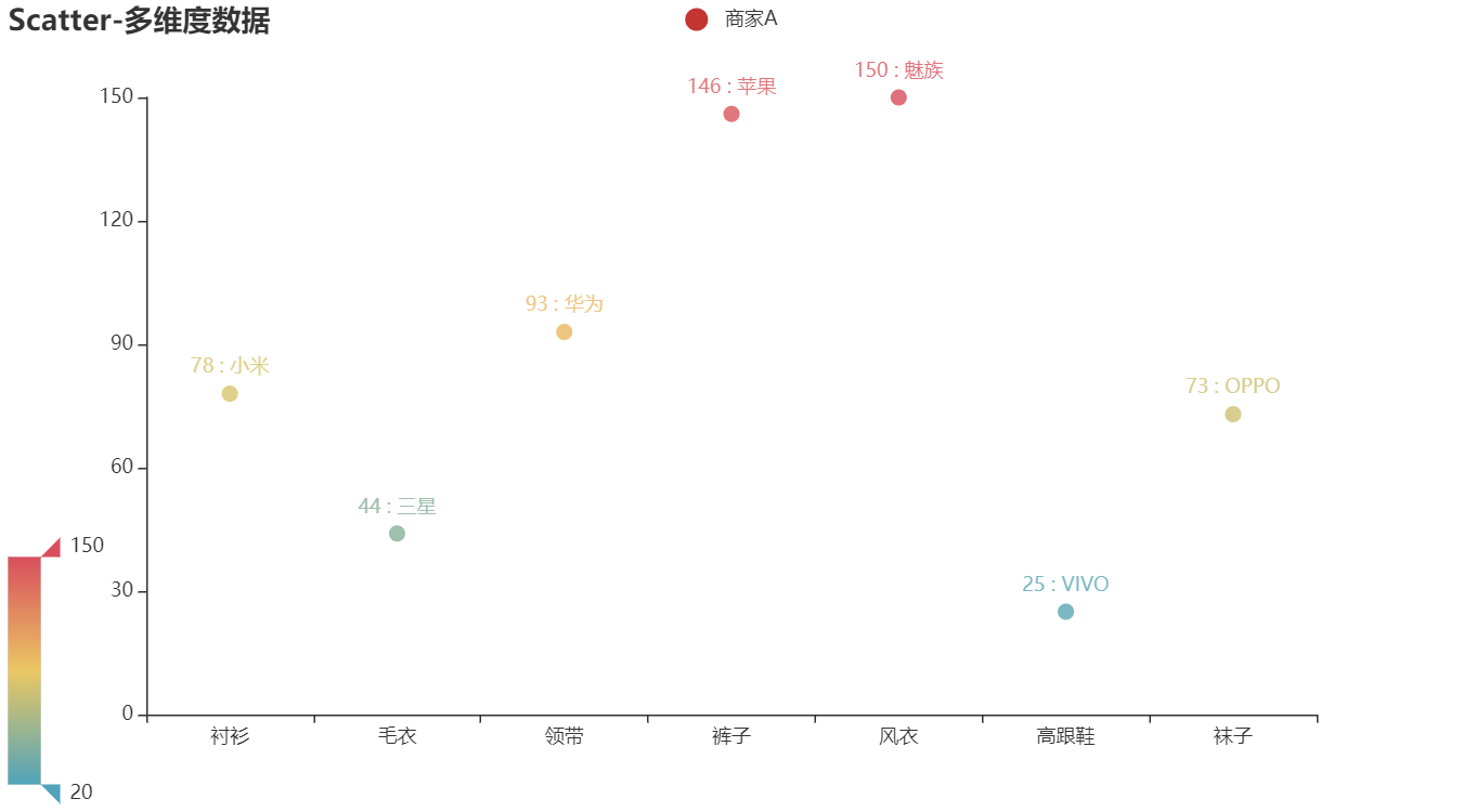
72.3 Scatter - Scatter_visualmap_color
from pyecharts import options as opts
from pyecharts.charts import Scatter
from pyecharts.faker import Faker

c = (
    Scatter()
    .add_xaxis(Faker.choose())
    .add_yaxis("商家A", Faker.values())
    .set_global_opts(
        title_opts=opts.TitleOpts(title="Scatter-VisualMap(Color)"),
        visualmap_opts=opts.VisualMapOpts(max_=150),
    )
    .render("scatter_visualmap_color.html")
)
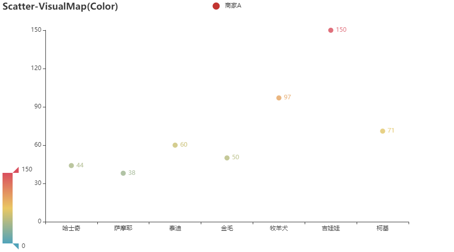
72.4 Scatter - Scatter_splitline
from pyecharts import options as opts
from pyecharts.charts import Scatter
from pyecharts.faker import Faker

c = (
    Scatter()
    .add_xaxis(Faker.choose())
    .add_yaxis("商家A", Faker.values())
    .set_global_opts(
        title_opts=opts.TitleOpts(title="Scatter-显示分割线"),
        xaxis_opts=opts.AxisOpts(splitline_opts=opts.SplitLineOpts(is_show=True)),
        yaxis_opts=opts.AxisOpts(splitline_opts=opts.SplitLineOpts(is_show=True)),
    )
    .render("scatter_splitline.html")
)
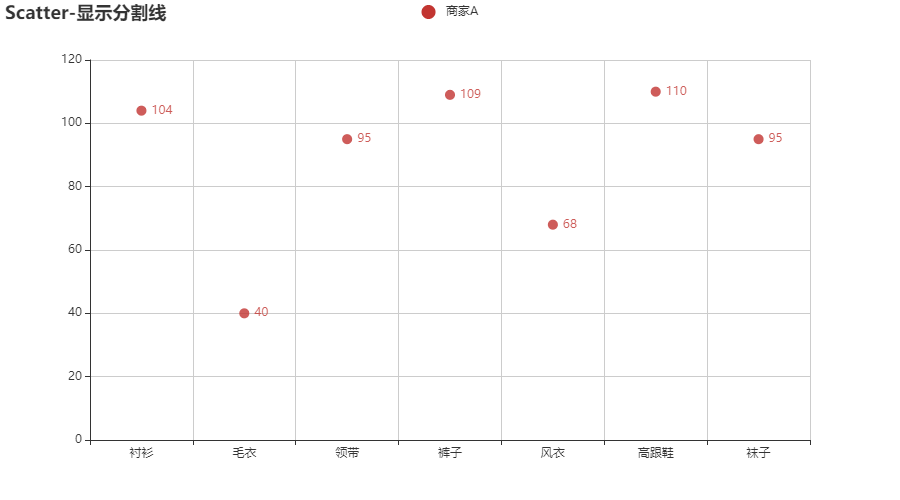
72.5 Scatter - Scatter_visualmap_size
from pyecharts import options as opts
from pyecharts.charts import Scatter
from pyecharts.faker import Faker

c = (
    Scatter()
    .add_xaxis(Faker.choose())
    .add_yaxis("商家A", Faker.values())
    .add_yaxis("商家B", Faker.values())
    .set_global_opts(
        title_opts=opts.TitleOpts(title="Scatter-VisualMap(Size)"),
        visualmap_opts=opts.VisualMapOpts(type_="size", max_=150, min_=20),
    )
    .render("scatter_visualmap_size.html")
)

72.6 Season实践:VisualMapOpts(type_: str = “color”,“size”)
visualmap_opts=opts.VisualMapOpts(type_="size", max_=15, min_=0),
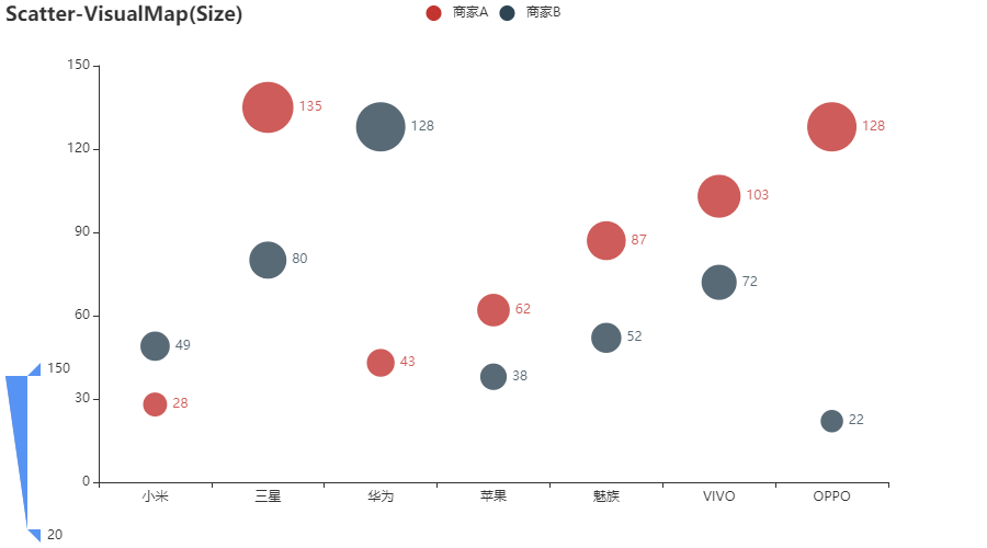
73.Overlap:层叠多图
73.1 Overlap - Overlap_bar_line
from pyecharts import options as opts
from pyecharts.charts import Bar, Line
from pyecharts.faker import Faker

v1 = [2.0, 4.9, 7.0, 23.2, 25.6, 76.7, 135.6, 162.2, 32.6, 20.0, 6.4, 3.3]
v2 = [2.6, 5.9, 9.0, 26.4, 28.7, 70.7, 175.6, 182.2, 48.7, 18.8, 6.0, 2.3]
v3 = [2.0, 2.2, 3.3, 4.5, 6.3, 10.2, 20.3, 23.4, 23.0, 16.5, 12.0, 6.2]


bar = (
    Bar()
    .add_xaxis(Faker.months)
    .add_yaxis("蒸发量", v1)
    .add_yaxis("降水量", v2)
    .extend_axis(
        yaxis=opts.AxisOpts(
            axislabel_opts=opts.LabelOpts(formatter="{value} °C"), interval=5
        )
    )
    .set_series_opts(label_opts=opts.LabelOpts(is_show=False))
    .set_global_opts(
        title_opts=opts.TitleOpts(title="Overlap-bar+line"),
        yaxis_opts=opts.AxisOpts(axislabel_opts=opts.LabelOpts(formatter="{value} ml")),
    )
)

line = Line().add_xaxis(Faker.months).add_yaxis("平均温度", v3, yaxis_index=1)
bar.overlap(line)
bar.render("overlap_bar_line.html")
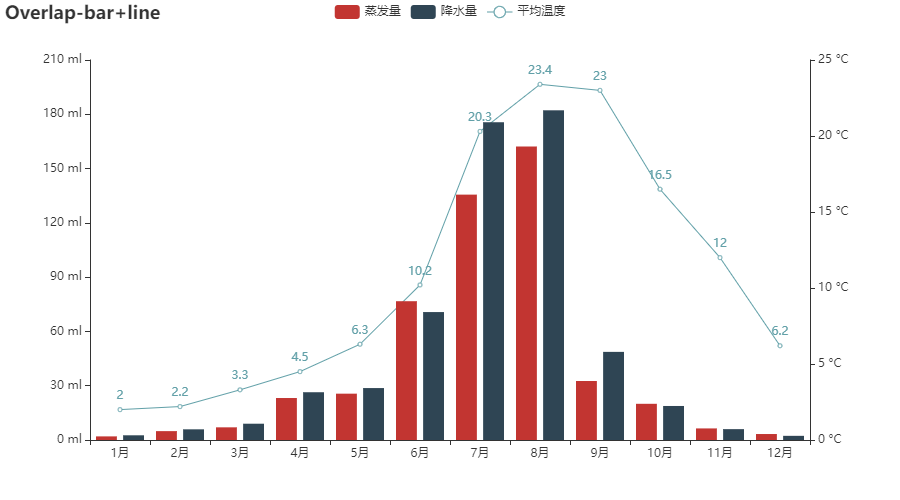
73.2 Overlap - Overlap_line_scatter
from pyecharts import options as opts
from pyecharts.charts import Line, Scatter
from pyecharts.faker import Faker

x = Faker.choose()
line = (
    Line()
    .add_xaxis(x)
    .add_yaxis("商家A", Faker.values())
    .add_yaxis("商家B", Faker.values())
    .set_global_opts(title_opts=opts.TitleOpts(title="Overlap-line+scatter"))
)
scatter = (
    Scatter()
    .add_xaxis(x)
    .add_yaxis("商家A", Faker.values())
    .add_yaxis("商家B", Faker.values())
)
line.overlap(scatter)
line.render("overlap_line_scatter.html")
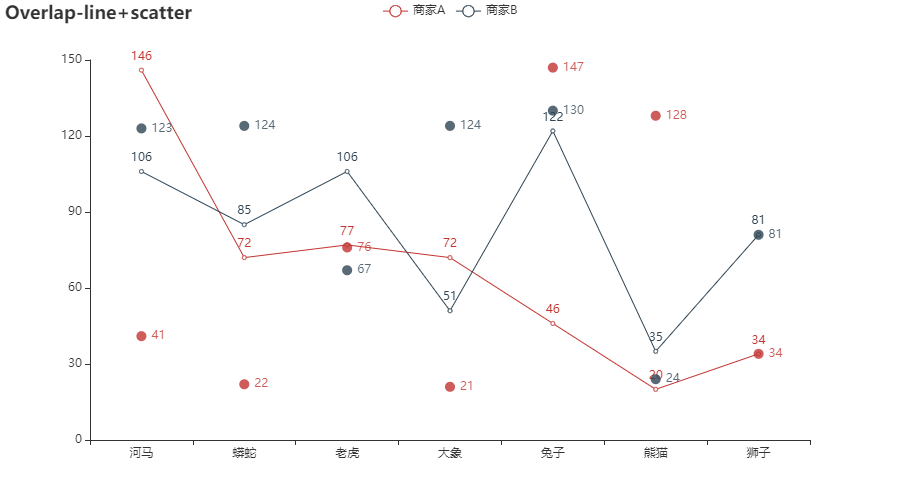


 被折叠的 条评论
为什么被折叠?
被折叠的 条评论
为什么被折叠?
 到【灌水乐园】发言


