Pandas - 订单数据分析和用户价值分群

一、数据准备

1、字段解释

orderID	订单ID
userID	用户ID
goodsID	商品ID
orderAmount	订单金额
payment	支付金额
channelID	销售渠道
platformType	支付方式
orderTime	下单时间
payTime	支付时间
chargeback	拒付

2、导入相应的包

import numpy as np
import pandas as pd
import matplotlib.pyplot as plt

plt.rcParams['font.sans-serif'].insert(0, 'SimHei')
plt.rcParams['axes.unicode_minus'] = False
%config InlineBackend.figure_format = 'svg'

 3、读如数据并且用index_col='id'将id设为索引列，读出数据10万条

orders_df = pd.read_excel('data/某电商平台2021年订单数据.xlsx',index_col='id')
orders_df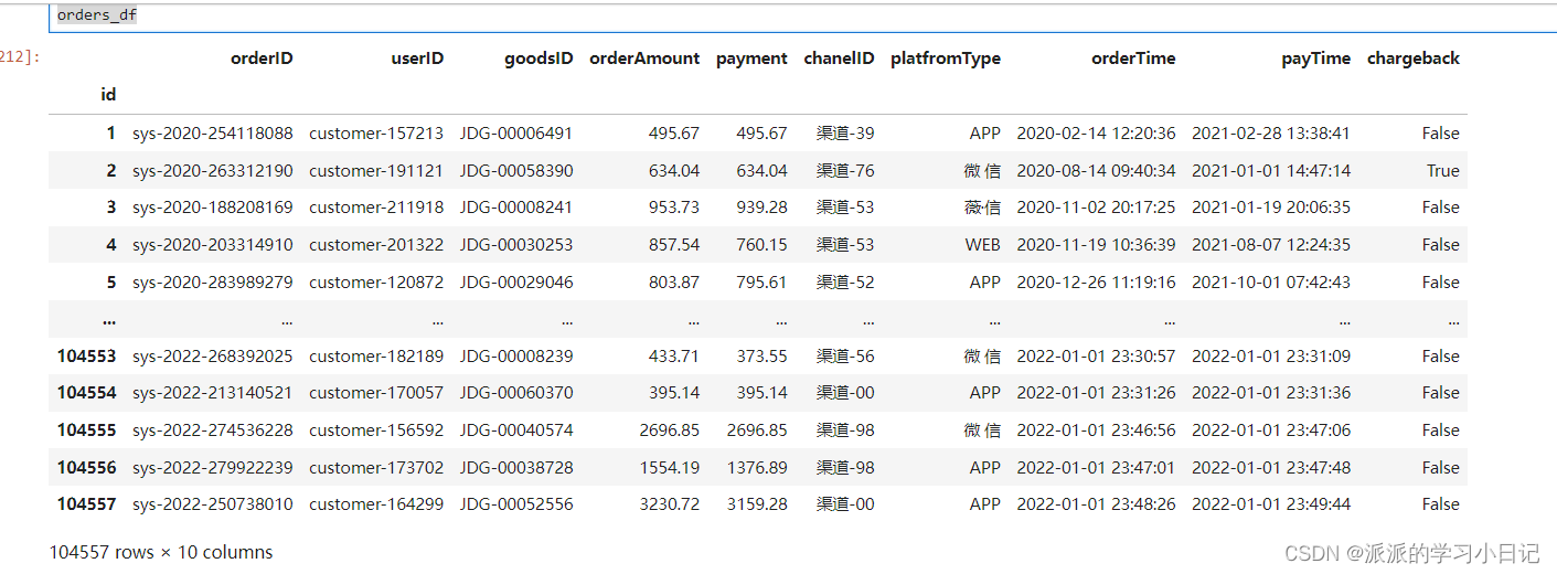

4、修改渠道字段的列名为channelID，平台字段的列名为platformType

orders_df.rename(columns={'chanelID':'channelID','platfromType':'platformType'},inplace=True)

5、筛选出2021年的订单（orderTime在2021年）

先将年份不在2021年的数据的数据索引获取出来再在原表中删除将其对应的索引。

index = orders_df[orders_df.orderTime.dt.year != 2021].index
orders_df.drop(index = index,inplace=True)

 6、删除支付金额（payment）小于0的订单，删除支付金额（payment）大于订单金额（orderAmount）的订单，删除支付时间（payTime）早于下单时间(orderTime)的订单，删除支付时长超过30分钟的订单

1）、先删除支付金额（payment）小于0的订单，和删除支付时间（payTime）早于下单时间(orderTime)的订单

index = orders_df[(orders_df.payment < 0) | (orders_df.payTime < orders_df.orderTime)].index
orders_df.drop(index = index,inplace= True)
orders_df

 2）删除支付时长超过30分钟的订单

先将订单的支付时长按秒统计出来并且筛选

index = orders_df[(orders_df.payTime - orders_df.orderTime).dt.total_seconds() > 1800].index
orders_df.drop(index = index,inplace=True)

3)支付金额（payment）大于订单金额（orderAmount）的订单,将支付金额修改为订单金额乘以平均折扣

先算出订单的平均折扣率

a,b = orders_df[orders_df.payment <= orders_df.orderAmount][['orderAmount','payment']].sum()
mean_discount = b / a

发现折扣率基本在0.95上。最后用where将支付金额进行修改

# Series.where - 满足条件的保留原来的值,不满足条件用第二个参数值
# Series.mask - 满足条件的被替换掉，不满足条件保留原来的值
orders_df['payment'] = orders_df.payment.where(
    orders_df.payment <= orders_df.orderAmount,
    (orders_df.orderAmount * mean_discount).round(2)
)

7、将渠道（channelID）字段的空值填充为众数

# 找出字段的众数在用fillna进行填充
mode_value = orders_df.channelID.mode()[0]
orders_df.channelID.fillna(mode_value,inplace=True)
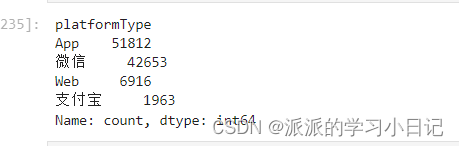
orders_df.info()

8、处理掉平台（platformType）字段的异常值（最后只有四种值：微信、支付宝、App、Web）

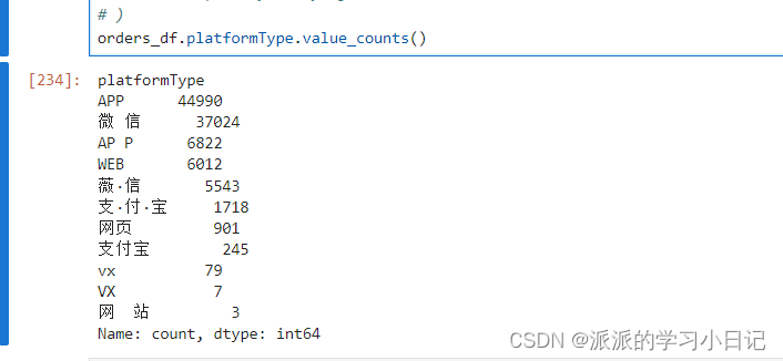
orders_df['platformType'] = orders_df.platformType.str.replace(
    r'[·\s]','',regex = True
).str.title().replace(
    r'薇信|Vx','微信',regex = True
).str.replace(
    r'网页|网站','Web',regex = True
)

 

二、数据分析

1、统计出核心指标，包括：GMV、净销售额、客单价、拒退率、复购率

GVM = orders_df.orderAmount.sum()
sales = orders_df.query('not chargeback').payment.sum()
# 客单价 用户数量进行去重nunique()
arppu = sales / orders_df.userID.nunique()
brate = orders_df.query('chargeback').orderID.count() / orders_df.orderID.nunique()

temp = pd.pivot_table(
    orders_df.query('not chargeback'),
    index = 'userID',
    values = 'orderID',
    aggfunc='nunique'
).rename(columns= {'orderID':'orderCount'})
ser = temp.orderCount.map(lambda x: 1 if x > 1 else 0)
rrate = ser.sum() / ser.count()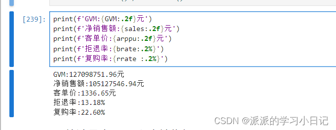

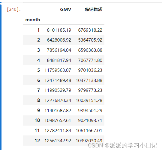
2、 统计月度GMV和净销售额

先分别创建

temp1 = pd.pivot_table(
    orders_df,
    index = 'month',
    values= 'orderAmount',
    aggfunc='sum'
).rename(columns={'orderAmount':'GMV'})
temp2 = pd.pivot_table(
    orders_df.query('not chargeback'),
    index = 'month',
    values = 'payment',
    aggfunc = 'sum'
).round(2).rename(columns={'payment':'净销售额'})
# temp = pd.concat((temp1,temp2),axis = 1)
temp = pd.merge(temp1,temp2,how = 'inner',left_index = True,right_index= True)
temp

两个指标的透视表在用merge对数据进行重塑

对数据进行可视化

temp.plot(kind = 'line',figsize = (10,4),marker = '*',linewidth = 0.5,linestyle = '--')
plt.ylim(0,14000000)
plt.xticks(temp.index)
plt.legend(loc = 'lower right')
plt.show()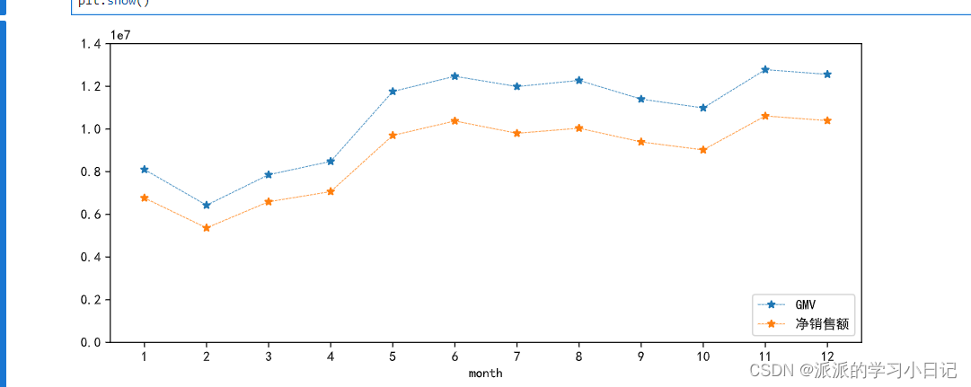

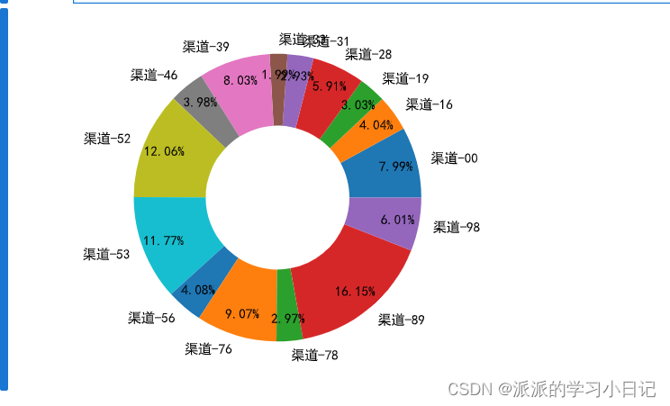
3、统计各渠道对流量（订单量）的贡献占比

先创建透视表 

temp5 = orders_df.pivot_table(
    index = 'channelID',
    values= 'orderID',
    aggfunc='count'
).rename(columns={'orderID':'orderID_count'})
temp5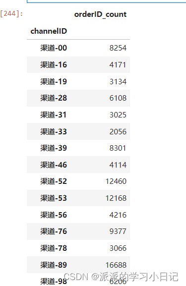

数据进行可视化

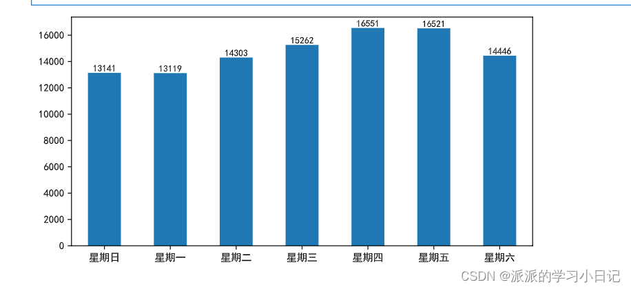
4、 统计星期几用户下单量最高

 先用weekday找出星期几并且添加

orders_df['weekday'] = (orders_df.orderTime.dt.weekday + 1) % 7

tem4 = orders_df.pivot_table(
    index='weekday',
    values='orderID',
    aggfunc='nunique'
)
temp4.plot(kind='bar', figsize=(8, 4), xlabel='', legend=False)
for i in np.arange(7):
    plt.text(i, temp4.orderID[i] + 100, temp4.orderID[i], ha='center', fontdict=dict(size=9))
plt.xticks(np.arange(7), labels=[f'星期{x}' for x in '日一二三四五六'], rotation=0)
plt.show()

5、 统计每天哪个时段用户下单量最高 

先对时间用对时间字段进行向下取整，并提出时间的时分

orders_df['time'] = orders_df.orderTime.dt.floor('30T').dt.strftime('%H:%M')
temp6 = pd.pivot_table(
    orders_df,
    index = 'time',
    values='orderID',
    aggfunc='nunique'
)
plt.figure(figsize=(10,4),dpi = 200)
plt.bar(temp6.index,temp6.orderID,color = np.random.random((8,3)),width  = 0.5)
plt.xticks(rotation = 75)
plt.show()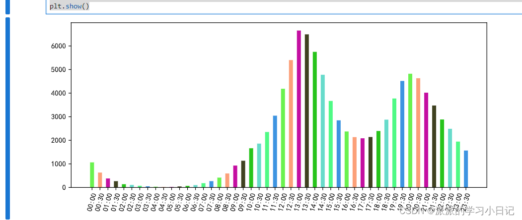

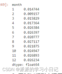
6、以自然月为窗口计算每个月的复购率

直接创建透视表

temp7 = pd.pivot_table(
    orders_df.query('not chargeback'),
    columns='month',
    index = 'userID',
    values = 'orderID',
    aggfunc='nunique'
)
temp7 = temp7.map(lambda x: x if np.isnan(x) else (1 if x > 1 else 0))
temp7.sum()/temp7.count()
# temp7.sum()有复购行为的人数，temp7.count()有购买行为的人数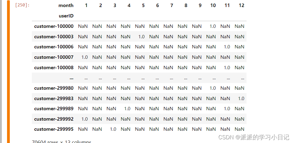

8、用RFM模型实现用户价值分群

1、r recency:用户的新近性，最后一次消费时间体现。
2、f frequency:用户的消费频率
3、m monetary：用户的消费金额

所以这里直接创建的是透视表对orderTim下单时间求最大值作为用户消费的最近时间R,'orderID'订单编号用count计算用户的消费频率F，用sum计算'payment'用户的总消费金额M

rfm_model_df = pd.pivot_table(
    orders_df.query('not chargeback'),
    index = 'userID',
    values=['orderTime','orderID','payment'],
    aggfunc={
        'orderTime':'max',
        'orderID':'nunique',
        'payment':'sum'
    }
).rename(columns={'orderTime':'R','orderID':'F','payment':'M'})
rfm_model_df

在计算出用户距离2021年12月31日59时59分的间隔天数,再对列进行排序

from datetime import datetime
rfm_model_df['R'] = (datetime(2021,12,31,23,59,59) - rfm_model_df.R).dt.days
# reindex- 调整行索引或列索引的顺序（也可用花式索引来调整）
rfm_model_df = rfm_model_df.reindex(columns=['R','F','M'])
rfm_model_df

将RFM模型的原始数据处理为对应的等级

def handle_r(value):
    if value <= 14:
        return 5
    elif value <= 30:
        return 4
    elif value <= 90:
        return 3
    elif value <= 180:
        return 2
    return 1
def handle_f(value):
    if value >= 5:
        return 5
    return value
def handle_m(value):
    if value < 500:
        return 1
    elif value < 800:
        return 2
    elif value < 1200:
        return 3
    elif value < 2500:
        return 4
    return 5

使用 apply() 方法将 handle_r、 handle_f、handle_m函数应用到 R 列的每一个值上，并将处理后的值赋值回 rfm_model_df 中的 R、F、M列

rfm_model_df['R'] = rfm_model_df.R.apply(handle_r)
rfm_model_df['F'] = rfm_model_df.F.apply(handle_f)
rfm_model_df['M'] = rfm_model_df.M.apply(handle_m)

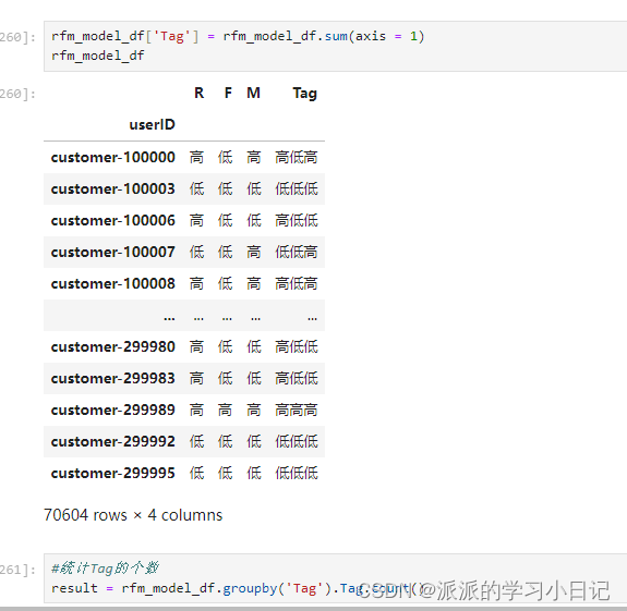
 Pandas 的 map() 函数和 lambda 表达式，将每一列中高于平均值的数据点替换为 ‘高’，低于平均值的数据点替换为 ‘低’。

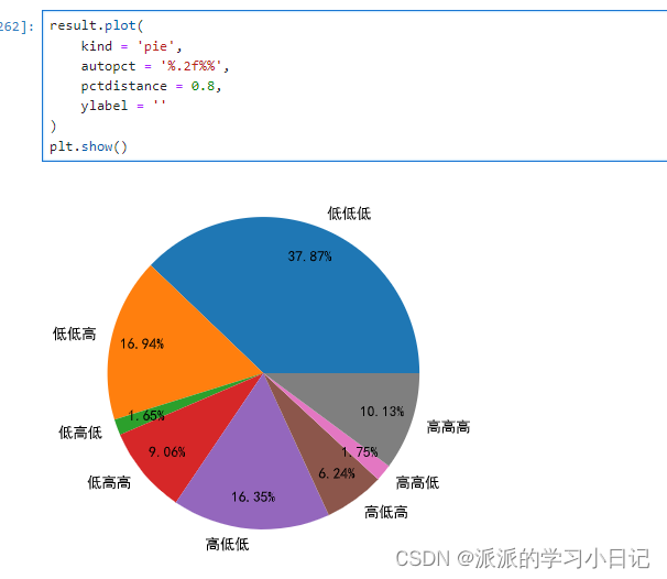
对群体打上标签并对不同的客户群体进行计数判断客户的价值