卷积神经网络(CNN)详解与代码实现

1.应用场景

卷积神经网络的应用不可谓不广泛，主要有两大类，数据预测和图片处理。数据预测自然不需要多说，图片处理主要包含有图像分类，检测，识别，以及分割方面的应用。
图像分类：场景分类，目标分类
图像检测：显著性检测，物体检测，语义检测等等
图像识别：人脸识别，字符识别，车牌识别，行为识别，步态识别等等
图像分割：前景分割，语义分割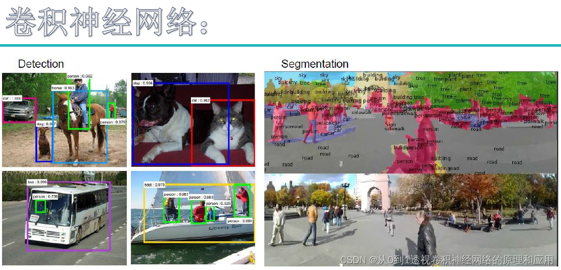

2.卷积神经网络结构

卷积神经网络主要是由输入层、卷积层、激活函数、池化层、全连接层、损失函数组成，表面看比较复杂，其实质就是特征提取以及决策推断。
要使特征提取尽量准确，就需要将这些网络层结构进行组合，比如经典的卷积神经网络模型AlexNet:5个卷积层+3个池化层+3个连接层结构。
2.1 卷积（convolution）
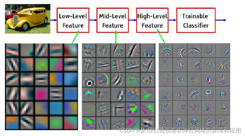
卷积的作用就是提取特征，因为一次卷积可能提取的特征比较粗糙，所以多次卷积，以及层层纵深卷积，层层提取特征（千万要区别于多次卷积，因为每一层里含有多次卷积）。
这里可能就有小伙伴问：为什么要进行层层纵深卷积，而且还要每层多次？
你可以理解为物质A有自己的多个特征（高、矮、胖、瘦、、、），所以在物质A上需要多次提取，得到不同的特征，然后这些特征组合后发生化学反应生成物质B，而物质B又有一些新的专属于自己的特征，所以需要进一步卷积。这是我个人的理解，不对的话或者有更形象的比喻还请不吝赐教啊。

在卷积层中，每一层的卷积核是不一样的。比如AlexNet
第一层：961111（96表示卷积核个数，11表示卷积核矩阵宽高） stride（步长） = 4 pad（边界补零） = 0
第二层：25655 stride（步长） = 1 pad（边界补零） = 2
第三，四层：38433 stride（步长） = 1 pad（边界补零） = 1
第五层：25633 stride（步长） = 1 pad（边界补零） = 2
卷积的篇幅说了这么多，那么到底是如何进行运算的呢，虽说网络上关于卷积运算原理铺天盖地，但是个人总感觉讲得不够透彻，或者说本人智商有待提高，希望通过如下这幅图（某位大神的杰作）来使各位看官们能够真正理解。

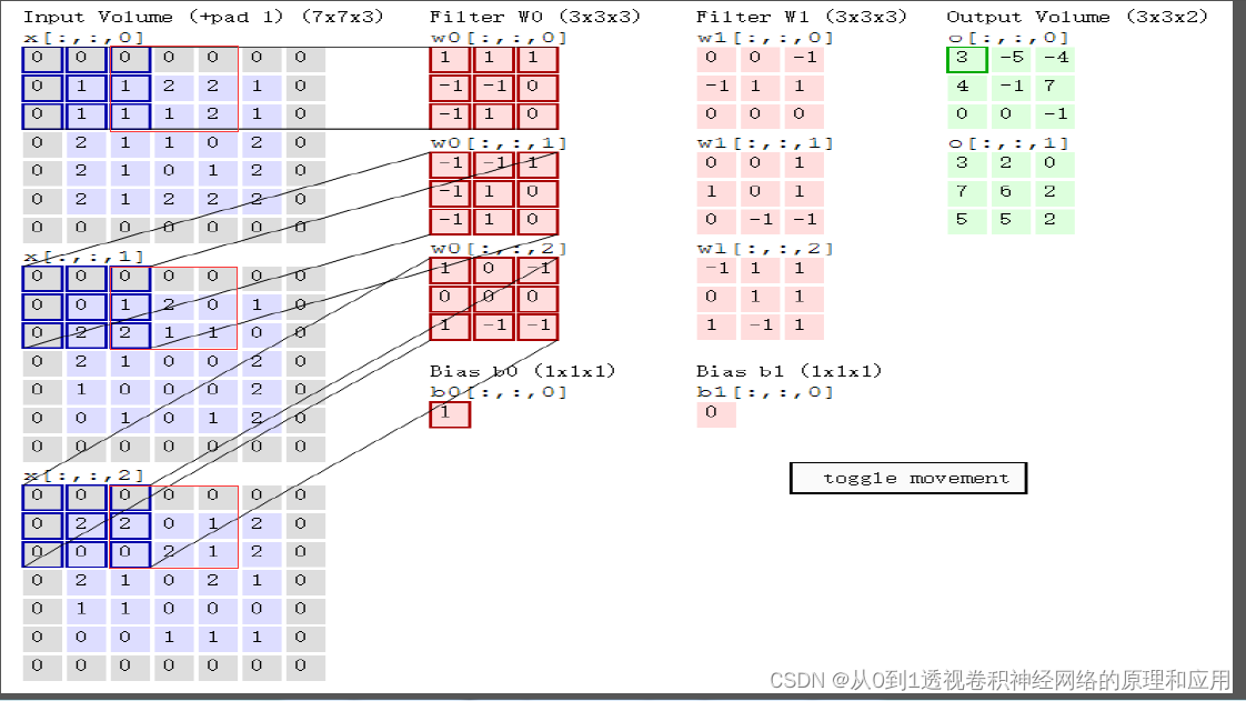
这里举的例子是一个输入图片（553），卷积核（333），有两个（Filter W0，W1），偏置b也有两个（Bios b0，b1），卷积结果Output Volumn（332），步长stride = 2。
输入：773 是因为 pad = 1 （在图片边界行和列都补零，补零的行和的数目是1），（对于彩色图片，一般都是RGB3种颜色，号称3通道，77指图片高h * 宽w），补零的作用是能够提取图片边界的特征。
卷积核深度为什么要设置成3呢？这是因为输入是3通道，所以卷积核深度必须与输入的深度相同。至于卷积核宽w，高h则是可以变化的，但是宽高必须相等。
卷积核输出o[0,0,0] = 3 （Output Volumn下浅绿色框结果），这个结果是如何得到的呢？ 其实关键就是矩阵对应位置相乘再相加（千万不要跟矩阵乘法搞混淆啦）
=> w0[:,:,0] * x[:,:,0]蓝色区域矩阵(R通道) + w0[:,:,1] * x[:,:,1]蓝色区域矩阵（G通道）+ w0[:,:,2] * x[:,:,2]蓝色区域矩阵（B通道） + b0（千万不能丢，因为 y = w * x + b）

第一项 => 0 * 1 + 0 * 1 + 0 * 1 + 0 * (-1) + 1 * (-1) + 1 * 0 + 0 * (-1) + 1 * 1 + 1 * 0 = 0

第二项 => 0 * (-1) + 0 * (-1) + 0 * 1 + 0 * (-1) + 0 * 1 + 1 * 0 + 0 * (-1) + 2 * 1 + 2 * 0 = 2

第三项 => 0 * 1 + 0 * 0 + 0 * (-1) + 0 * 0 + 2 * 0 + 2 * 0 + 0 * 1 + 0 * (-1) + 0 * (-1) = 0

卷积核输出o[0,0,0] = > 第一项 + 第二项 + 第三项 + b0 = 0 + 2 + 0 + 1 = 3

o[0,0,1] = -5 又是如何得到的呢？

因为这里的stride = 2 ，所以 输入的窗口就要滑动两个步长，也就是红色框的区域，而运算跟之前是一样的

第一项 => 0 * 1 + 0 * 1 + 0 * 1 + 1 * (-1) + 2 * (-1) + 2 * 0 + 1 * (-1) + 1 * 1 + 2 * 0 = -3

第二项 => 0 * (-1) + 0 * (-1) + 0 * 1 + 1 * (-1) + 2 * 1 + 0 * 0 + 2 * (-1) + 1 * 1 + 1 * 0 = 0

第三项 => 0 * 1 + 0 * 0 + 0 * (-1) + 2 * 0 + 0 * 0 + 1 * 0 + 0 * 1 + 2 * (-1) + 1 * (-1) = - 3

卷积核输出o[0,0,1] = > 第一项 + 第二项 + 第三项 + b0 = (-3) + 0 + (-3) + 1 = -5

之后以此卷积核窗口大小在输入图片上滑动，卷积求出结果，因为有两个卷积核，所有就有两个输出结果。

这里小伙伴可能有个疑问，输出窗口是如何得到的呢？

这里有一个公式：输出窗口宽 w = (输入窗口宽 w - 卷积核宽 w + 2 * pad)/stride + 1 ，输出高 h = 输出窗口宽 w

以上面例子， 输出窗口宽 w = ( 5 - 3 + 2 * 1)/2 + 1 = 3 ，则输出窗口大小为 3 * 3，因为有2个输出，所以是 332。

2.2 Relu激活函数

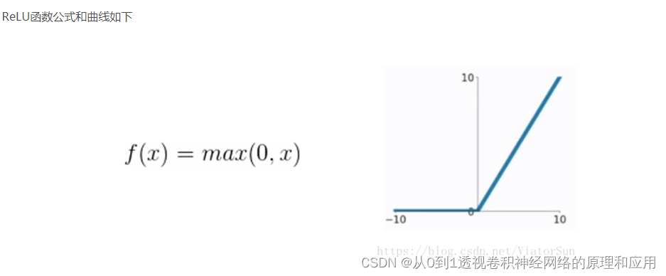
相信看过卷积神经网络结构（CNN）的伙伴们都知道，激活函数无处不在，特别是CNN中，在卷积层后，全连接（FC）后都有激活函数Relu的身影，
那么这就自然不得不让我们产生疑问：
问题1、为什么要用激活函数？它的作用是什么？
问题2、在CNN中为什么要用Relu，相比于sigmoid，tanh，它的优势在什么地方？
对于第1个问题：由 y = w * x + b 可知，如果不用激活函数，每个网络层的输出都是一种线性输出，而我们所处的现实场景，其实更多的是各种非线性的分布。
这也说明了激活函数的作用是将线性分布转化为非线性分布，能更逼近我们的真实场景。
对于第2个问题： 先看sigmoid，tanh分布

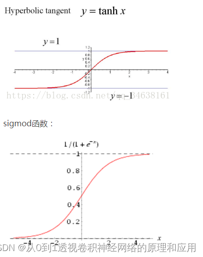
他们在 x -> 时，输出就变成了恒定值，因为求梯度时需要对函数求一阶偏导数，而不论是sigmoid，还是tanhx，他们的偏导都为0，也就是存在所谓的梯度消失问题，最终也就会导致权重参数w ， b 无法更新。相比之下，Relu就不存在这样的问题，另外在 x > 0 时，Relu求导 = 1，这对于反向传播计算dw，db，是能够大大的简化运算的。
使用sigmoid还会存在梯度爆炸的问题，比如在进行前向传播和反向传播迭代次数非常多的情况下，sigmoid因为是指数函数，其结果中

某些值会在迭代中累积，并成指数级增长，最终会出现NaN而导致溢出。

2.3 池化
池化层一般在卷积层+ Relu之后，它的作用是：

1、减小输入矩阵的大小（只是宽和高，而不是深度），提取主要特征。（不可否认的是，在池化后，特征会有一定的损失，所以，有些经典模型就去掉了池化这一层）。

它的目的是显而易见的，就是在后续操作时能降低运算。

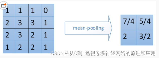
2、一般采用mean_pooling（均值池化）和max_pooling（最大值池化），对于输入矩阵有translation（平移），rotation（旋转），能够保证特征的不变性。

mean_pooling 就是输入矩阵池化区域求均值，这里要注意的是池化窗口在输入矩阵滑动的步长跟stride有关，一般stride = 2.（图片是直接盗过来，这里感谢原创）

最右边7/4 => (1 + 1 + 2 + 3)/4

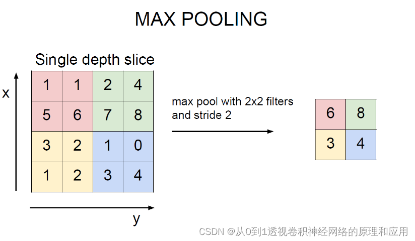
max_pooling 最大值池化，就是每个池化区域的最大值放在输出对应位置上。

2.4 全连接（full connection）
作用：分类器角色，将特征映射到样本标记空间，本质是矩阵变换（affine）。

至于变换的实现见后面的代码流程图，或者最好是跟一下代码，这样理解更透彻。

2.5 损失函数（softmax_loss）
作用：计算损失loss，从而求出梯度grad。

常用损失函数有:MSE均方误差，SVM（支持向量机）合页损失函数，Cross Entropy交叉熵损失函数。

这几种损失函数目前还看不出谁优谁劣，估计只有在具体的应用场景中去验证了。至于这几种损失函数的介绍，

大家可以去参考《常用损失函数小结》https://blog.csdn.net/zhangjunp3/article/details/80467350，这个哥们写得比较详细。

在后面的代码实例中，用到的是softmax_loss，它属于Cross Entropy交叉熵损失函数。

softmax计算公式：

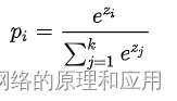
其中， 是要计算的类别 的网络输出，分母是网络输出所有类别之和（共有 个类别）， 表示第 类的概率。

交叉熵损失：

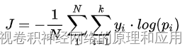
其中， 是类别 的真实标签， 表示第 类的概率， 是样本总数， 是类别数。

其中 表示真实标签对应索引下预测的目标值， 类别索引。

这个有点折磨人，原理讲解以及推导请大家可以参考这位大神的博客：http://www.cnblogs.com/zongfa/p/8971213.html。

2.6 前向传播（forward propagation）
前向传播包含之前的卷积，Relu激活函数，池化（pool），全连接(fc)，可以说，在损失函数之前操作都属于前向传播。

主要是权重参数w , b 初始化，迭代，以及更新w, b,生成分类器模型。

2.7 反向传播（back propagation）
反向传播包含损失函数，通过梯度计算dw，db，Relu激活函数逆变换，反池化，反全连接。

2.8 随机梯度下降（sgd_momentum）
作用：由梯度grad计算新的权重矩阵w

sgd公式：

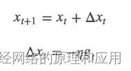
其中，η为学习率，gt为x在t时刻的梯度。

一般我们是将整个数据集分成n个epoch，每个epoch再分成m个batch，每次更新都利用一个batch的数据，而非整个训练集。

优点：batch的方法可以减少机器的压力，并且可以更快地收敛。

缺点：其更新方向完全依赖于当前的batch，因而其更新十分不稳定。

为了解决这个问题，momentum就横空出世了，具体原理详解见下路派出所（这名字霸气）的博客http://www.cnblogs.com/callyblog/p/8299074.html。

momentum即动量，它模拟的是物体运动时的惯性，即更新的时候在一定程度上保留之前更新的方向，同时利用当前batch的梯度微调最终的更新方向。

这样一来，可以在一定程度上增加稳定性，从而学习地更快，并且还有一定摆脱局部最优的能力：

其中，ρ 即momentum，表示要在多大程度上保留原来的更新方向，这个值在0-1之间，在训练开始时，由于梯度可能会很大，所以初始值一般选为0.5；

当梯度不那么大时，改为0.9。η 是学习率，即当前batch的梯度多大程度上影响最终更新方向，跟普通的SGD含义相同。ρ 与 η 之和不一定为1。

3.代码实现流程图以及介绍
代码流程图：费了老大劲，终于弄完了，希望对各位看官们有所帮助，建议对比流程图和跟踪代码，加深对原理的理解。

特别是前向传播和反向传播维度的变换，需要重点关注。

4.代码实现

当然，代码的整个实现是某位大神实现的，我只是在上面做了些小改动以及重点函数做了些注释，有不妥之处也希望大家不吝指教。

因为原始图片数据集太大，不好上传，大家可以直接在http://www.cs.toronto.edu/~kriz/cifar.html下载CIFAR-10 python version，
有163M，放在代码文件同路径下即可。

cnn.py

# -*- coding: utf-8 -*-
import matplotlib.pyplot as plt
'''同路径下py模块引用'''

try:
    from . import data_utils
    from . import solver
    from . import cnn
except Exception:
    import data_utils
    import solver
    import cnn

import numpy as np
# 获取样本数据
data = data_utils.get_CIFAR10_data()
# model初始化（权重因子以及对应偏置 w1,b1 ,w2,b2 ,w3,b3，数量取决于网络层数）
model = cnn.ThreeLayerConvNet(reg=0.9)
solver = solver.Solver(model, data,
                lr_decay=0.95,
                print_every=10, num_epochs=5, batch_size=2,
                update_rule='sgd_momentum',
                optim_config={'learning_rate': 5e-4, 'momentum': 0.9})
# 训练，获取最佳model
solver.train()

plt.subplot(2, 1, 1)
plt.title('Training loss')
plt.plot(solver.loss_history, 'o')
plt.xlabel('Iteration')

plt.subplot(2, 1, 2)
plt.title('Accuracy')
plt.plot(solver.train_acc_history, '-o', label='train')
plt.plot(solver.val_acc_history, '-o', label='val')
plt.plot([0.5] * len(solver.val_acc_history), 'k--')
plt.xlabel('Epoch')
plt.legend(loc='lower right')
plt.gcf().set_size_inches(15, 12)
plt.show()


best_model = model
y_test_pred = np.argmax(best_model.loss(data['X_test']), axis=1)
y_val_pred = np.argmax(best_model.loss(data['X_val']), axis=1)
print ('Validation set accuracy: ',(y_val_pred == data['y_val']).mean())
print ('Test set accuracy: ', (y_test_pred == data['y_test']).mean())
# Validation set accuracy:  about 52.9%
# Test set accuracy:  about 54.7%


# Visualize the weights of the best network
"""
from vis_utils import visualize_grid

def show_net_weights(net):
    W1 = net.params['W1']
    W1 = W1.reshape(3, 32, 32, -1).transpose(3, 1, 2, 0)
    plt.imshow(visualize_grid(W1, padding=3).astype('uint8'))
    plt.gca().axis('off')
show_net_weights(best_model)
plt.show()
"""

data.utils.py

# -*- coding: utf-8 -*-
import pickle
import numpy as np
import os

#from scipy.misc import imread

def load_CIFAR_batch(filename):
  """ load single batch of cifar """
  with open(filename, 'rb') as f:
    datadict = pickle.load(f, encoding='bytes')
    X = datadict[b'data']
    Y = datadict[b'labels']
    X = X.reshape(10000, 3, 32, 32).transpose(0,2,3,1).astype("float")
    Y = np.array(Y)
    return X, Y

def load_CIFAR10(ROOT):
  """ load all of cifar """
  xs = []
  ys = []
  for b in range(1,2):
    f = os.path.join(ROOT, 'data_batch_%d' % (b, ))
    X, Y = load_CIFAR_batch(f)
    xs.append(X)
    ys.append(Y)
  Xtr = np.concatenate(xs)
  Ytr = np.concatenate(ys)
  del X, Y
  Xte, Yte = load_CIFAR_batch(os.path.join(ROOT, 'test_batch'))
  return Xtr, Ytr, Xte, Yte


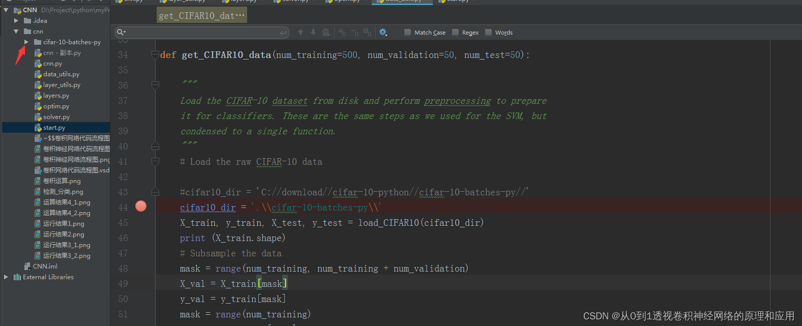
def get_CIFAR10_data(num_training=500, num_validation=50, num_test=50):

    """
    Load the CIFAR-10 dataset from disk and perform preprocessing to prepare
    it for classifiers. These are the same steps as we used for the SVM, but
    condensed to a single function.
    """
    # Load the raw CIFAR-10 data

    #cifar10_dir = 'C://download//cifar-10-python//cifar-10-batches-py//'
    cifar10_dir = '.\\cifar-10-batches-py\\'
    X_train, y_train, X_test, y_test = load_CIFAR10(cifar10_dir)
    print (X_train.shape)
    # Subsample the data
    mask = range(num_training, num_training + num_validation)
    X_val = X_train[mask]
    y_val = y_train[mask]
    mask = range(num_training)
    X_train = X_train[mask]
    y_train = y_train[mask]
    mask = range(num_test)
    X_test = X_test[mask]
    y_test = y_test[mask]

    # 标准化数据，求样本均值，然后 样本 - 样本均值，作用：使样本数据更收敛一些，便于后续处理
    # Normalize the data: subtract the mean image
    # 如果2维空间 m*n np.mean()后 => 1*n
    # 对于4维空间 m*n*k*j np.mean()后 => 1*n*k*j
    mean_image = np.mean(X_train, axis=0)
    X_train -= mean_image
    X_val -= mean_image
    X_test -= mean_image

    # 把通道channel 提前
    # Transpose so that channels come first
    X_train = X_train.transpose(0, 3, 1, 2).copy()
    X_val = X_val.transpose(0, 3, 1, 2).copy()
    X_test = X_test.transpose(0, 3, 1, 2).copy()

    # Package data into a dictionary
    return {
      'X_train': X_train, 'y_train': y_train,
      'X_val': X_val, 'y_val': y_val,
      'X_test': X_test, 'y_test': y_test,
    }

"""
def load_tiny_imagenet(path, dtype=np.float32):

  Load TinyImageNet. Each of TinyImageNet-100-A, TinyImageNet-100-B, and
  TinyImageNet-200 have the same directory structure, so this can be used
  to load any of them.

  Inputs:
  - path: String giving path to the directory to load.
  - dtype: numpy datatype used to load the data.

  Returns: A tuple of
  - class_names: A list where class_names[i] is a list of strings giving the
    WordNet names for class i in the loaded dataset.
  - X_train: (N_tr, 3, 64, 64) array of training images
  - y_train: (N_tr,) array of training labels
  - X_val: (N_val, 3, 64, 64) array of validation images
  - y_val: (N_val,) array of validation labels
  - X_test: (N_test, 3, 64, 64) array of testing images.
  - y_test: (N_test,) array of test labels; if test labels are not available
    (such as in student code) then y_test will be None.

  # First load wnids
  with open(os.path.join(path, 'wnids.txt'), 'r') as f:
    wnids = [x.strip() for x in f]

  # Map wnids to integer labels
  wnid_to_label = {wnid: i for i, wnid in enumerate(wnids)}

  # Use words.txt to get names for each class
  with open(os.path.join(path, 'words.txt'), 'r') as f:
    wnid_to_words = dict(line.split('\t') for line in f)
    for wnid, words in wnid_to_words.iteritems():
      wnid_to_words[wnid] = [w.strip() for w in words.split(',')]
  class_names = [wnid_to_words[wnid] for wnid in wnids]

  # Next load training data.
  X_train = []
  y_train = []
  for i, wnid in enumerate(wnids):
    if (i + 1) % 20 == 0:
      print 'loading training data for synset %d / %d' % (i + 1, len(wnids))
    # To figure out the filenames we need to open the boxes file
    boxes_file = os.path.join(path, 'train', wnid, '%s_boxes.txt' % wnid)
    with open(boxes_file, 'r') as f:
      filenames = [x.split('\t')[0] for x in f]
    num_images = len(filenames)

    X_train_block = np.zeros((num_images, 3, 64, 64), dtype=dtype)
    y_train_block = wnid_to_label[wnid] * np.ones(num_images, dtype=np.int64)
    for j, img_file in enumerate(filenames):
      img_file = os.path.join(path, 'train', wnid, 'images', img_file)
      img = imread(img_file)
      if img.ndim == 2:
        ## grayscale file
        img.shape = (64, 64, 1)
      X_train_block[j] = img.transpose(2, 0, 1)
    X_train.append(X_train_block)
    y_train.append(y_train_block)

  # We need to concatenate all training data
  X_train = np.concatenate(X_train, axis=0)
  y_train = np.concatenate(y_train, axis=0)

  # Next load validation data
  with open(os.path.join(path, 'val', 'val_annotations.txt'), 'r') as f:
    img_files = []
    val_wnids = []
    for line in f:
      img_file, wnid = line.split('\t')[:2]
      img_files.append(img_file)
      val_wnids.append(wnid)
    num_val = len(img_files)
    y_val = np.array([wnid_to_label[wnid] for wnid in val_wnids])
    X_val = np.zeros((num_val, 3, 64, 64), dtype=dtype)
    for i, img_file in enumerate(img_files):
      img_file = os.path.join(path, 'val', 'images', img_file)
      img = imread(img_file)
      if img.ndim == 2:
        img.shape = (64, 64, 1)
      X_val[i] = img.transpose(2, 0, 1)

  # Next load test images
  # Students won't have test labels, so we need to iterate over files in the
  # images directory.
  img_files = os.listdir(os.path.join(path, 'test', 'images'))
  X_test = np.zeros((len(img_files), 3, 64, 64), dtype=dtype)
  for i, img_file in enumerate(img_files):
    img_file = os.path.join(path, 'test', 'images', img_file)
    img = imread(img_file)
    if img.ndim == 2:
      img.shape = (64, 64, 1)
    X_test[i] = img.transpose(2, 0, 1)

  y_test = None
  y_test_file = os.path.join(path, 'test', 'test_annotations.txt')
  if os.path.isfile(y_test_file):
    with open(y_test_file, 'r') as f:
      img_file_to_wnid = {}
      for line in f:
        line = line.split('\t')
        img_file_to_wnid[line[0]] = line[1]
    y_test = [wnid_to_label[img_file_to_wnid[img_file]] for img_file in img_files]
    y_test = np.array(y_test)

  return class_names, X_train, y_train, X_val, y_val, X_test, y_test

"""
def load_models(models_dir):
  """
  Load saved models from disk. This will attempt to unpickle all files in a
  directory; any files that give errors on unpickling (such as README.txt) will
  be skipped.

  Inputs:
  - models_dir: String giving the path to a directory containing model files.
    Each model file is a pickled dictionary with a 'model' field.

  Returns:
  A dictionary mapping model file names to models.
  """
  models = {}
  for model_file in os.listdir(models_dir):
    with open(os.path.join(models_dir, model_file), 'rb') as f:
      try:
        models[model_file] = pickle.load(f)['model']
      except pickle.UnpicklingError:
        continue
  return models

layer.utils.py

# -*- coding: utf-8 -*-
try:
  from . import layers
except Exception:
  import layers




def affine_relu_forward(x, w, b):
  """
  Convenience layer that perorms an affine transform followed by a ReLU

  Inputs:
  - x: Input to the affine layer
  - w, b: Weights for the affine layer

  Returns a tuple of:
  - out: Output from the ReLU
  - cache: Object to give to the backward pass
  """
  a, fc_cache = layers.affine_forward(x, w, b)
  out, relu_cache = layers.relu_forward(a)
  cache = (fc_cache, relu_cache)
  return out, cache


def affine_relu_backward(dout, cache):
  """
  Backward pass for the affine-relu convenience layer
  """
  fc_cache, relu_cache = cache
  da = layers.relu_backward(dout, relu_cache)
  dx, dw, db = layers.affine_backward(da, fc_cache)
  return dx, dw, db


pass


def conv_relu_forward(x, w, b, conv_param):
  """
  A convenience layer that performs a convolution followed by a ReLU.

  Inputs:
  - x: Input to the convolutional layer
  - w, b, conv_param: Weights and parameters for the convolutional layer

  Returns a tuple of:
  - out: Output from the ReLU
  - cache: Object to give to the backward pass
  """
  a, conv_cache = layers.conv_forward_fast(x, w, b, conv_param)
  out, relu_cache = layers.relu_forward(a)
  cache = (conv_cache, relu_cache)
  return out, cache


def conv_relu_backward(dout, cache):
  """
  Backward pass for the conv-relu convenience layer.
  """
  conv_cache, relu_cache = cache
  da = layers.relu_backward(dout, relu_cache)
  dx, dw, db = layers.conv_backward_fast(da, conv_cache)
  return dx, dw, db


def conv_relu_pool_forward(x, w, b, conv_param, pool_param):
  """
  Convenience layer that performs a convolution, a ReLU, and a pool.

  Inputs:
  - x: Input to the convolutional layer
  - w, b, conv_param: Weights and parameters for the convolutional layer
  - pool_param: Parameters for the pooling layer

  Returns a tuple of:
  - out: Output from the pooling layer
  - cache: Object to give to the backward pass
  """
  a, conv_cache = layers.conv_forward_naive(x, w, b, conv_param)
  s, relu_cache = layers.relu_forward(a)
  out, pool_cache = layers.max_pool_forward_naive(s, pool_param)
  cache = (conv_cache, relu_cache, pool_cache)
  return out, cache


def conv_relu_pool_backward(dout, cache):
  """
  Backward pass for the conv-relu-pool convenience layer
  """
  conv_cache, relu_cache, pool_cache = cache
  ds = layers.max_pool_backward_naive(dout, pool_cache)
  da = layers.relu_backward(ds, relu_cache)
  dx, dw, db = layers.conv_backward_naive(da, conv_cache)
  return dx, dw, db

layers.py

import numpy as np

'''
全连接层：矩阵变换，获取对应目标相同的行与列
输入x: 2*32*16*16
输入x_row: 2*8192
超参w：8192*100
输出：矩阵乘法 2*8192 ->8192*100 =>2*100
'''
def affine_forward(x, w, b):
    """
    Computes the forward pass for an affine (fully-connected) layer.
    The input x has shape (N, d_1, ..., d_k) and contains a minibatch of N
    examples, where each example x[i] has shape (d_1, ..., d_k). We will
    reshape each input into a vector of dimension D = d_1 * ... * d_k, and
    then transform it to an output vector of dimension M.
    Inputs:
    - x: A numpy array containing input data, of shape (N, d_1, ..., d_k)
    - w: A numpy array of weights, of shape (D, M)
    - b: A numpy array of biases, of shape (M,)
    Returns a tuple of:
    - out: output, of shape (N, M)
    - cache: (x, w, b)
    """
    out = None
    # Reshape x into rows
    N = x.shape[0]
    x_row = x.reshape(N, -1)         # (N,D) -1表示不知道多少列，指定行，就能算出列 = 2 * 32 * 16 * 16/2 = 8192
    out = np.dot(x_row, w) + b       # (N,M) 2*8192 8192*100 =>2 * 100
    cache = (x, w, b)

    return out, cache
'''
反向传播之affine矩阵变换
根据dout求出dx,dw,db
由 out = w * x =>
dx = dout * w
dw = dout * x
db = dout * 1
因为dx 与 x，dw 与 w，db 与 b 大小（维度）必须相同
dx = dout * wT  矩阵乘法
dw = dxT * dout 矩阵乘法
db = dout 按列求和
'''
def affine_backward(dout, cache):
    """
    Computes the backward pass for an affine layer.
    Inputs:
    - dout: Upstream derivative, of shape (N, M)
    - cache: Tuple of:
    - x: Input data, of shape (N, d_1, ... d_k)
    - w: Weights, of shape (D, M)
    Returns a tuple of:
    - dx: Gradient with respect to x, of shape (N, d1, ..., d_k)
      dx = dout * w
    - dw: Gradient with respect to w, of shape (D, M)
      dw = dout * x
    - db: Gradient with respect to b, of shape (M,)
      db = dout * 1
    """

    x, w, b = cache
    dx, dw, db = None, None, None
    dx = np.dot(dout, w.T)                       # (N,D)
    # dx维度必须跟x维度相同
    dx = np.reshape(dx, x.shape)                 # (N,d1,...,d_k)
    # 转换成二维矩阵
    x_row = x.reshape(x.shape[0], -1)            # (N,D)
    dw = np.dot(x_row.T, dout)                   # (D,M)

    db = np.sum(dout, axis=0, keepdims=True)     # (1,M)

    return dx, dw, db

def relu_forward(x):
    """ 激活函数，解决sigmoid梯度消失问题，网络性能比sigmoid更好
    Computes the forward pass for a layer of rectified linear units (ReLUs).
    Input:
    - x: Inputs, of any shape
    Returns a tuple of:
    - out: Output, of the same shape as x
    - cache: x
    """
    out = None
    out = ReLU(x)
    cache = x

    return out, cache

def relu_backward(dout, cache):
    """
    Computes the backward pass for a layer of rectified linear units (ReLUs).
    Input:
    - dout: Upstream derivatives, of any shape
    - cache: Input x, of same shape as dout
    Returns:
    - dx: Gradient with respect to x
    """
    dx, x = None, cache
    dx = dout
    dx[x <= 0] = 0

    return dx

def svm_loss(x, y):
    """
    Computes the loss and gradient using for multiclass SVM classification.
    Inputs:
    - x: Input data, of shape (N, C) where x[i, j] is the score for the jth class
         for the ith input.
    - y: Vector of labels, of shape (N,) where y[i] is the label for x[i] and
         0 <= y[i] < C
    Returns a tuple of:
    - loss: Scalar giving the loss
    - dx: Gradient of the loss with respect to x
    """
    N = x.shape[0]
    correct_class_scores = x[np.arange(N), y]
    margins = np.maximum(0, x - correct_class_scores[:, np.newaxis] + 1.0)
    margins[np.arange(N), y] = 0
    loss = np.sum(margins) / N
    num_pos = np.sum(margins > 0, axis=1)
    dx = np.zeros_like(x)
    dx[margins > 0] = 1
    dx[np.arange(N), y] -= num_pos
    dx /= N

    return loss, dx
'''
softmax_loss 求梯度优点: 求梯度运算简单，方便
softmax: softmax用于多分类过程中，它将多个神经元的输出，映射到（0,1）区间内，
可以看成概率来理解，从而来进行多分类。
Si = exp(i)/[exp(j)求和]
softmax_loss：损失函数，求梯度dx必须用到损失函数，通过梯度下降更新超参
Loss = -[Ypred*ln(Sj真实类别位置的概率值)]求和
梯度dx : 对损失函数求一阶偏导
如果 j = i =>dx = Sj - 1
如果 j != i => dx = Sj
'''
def softmax_loss(x, y):
    """
    Computes the loss and gradient for softmax classification.    Inputs:
    - x: Input data, of shape (N, C) where x[i, j] is the score for the jth class
    for the ith input.
    - y: Vector of labels, of shape (N,) where y[i] is the label for x[i] and
         0 <= y[i] < C
    Returns a tuple of:
    - loss: Scalar giving the loss
    - dx: Gradient of the loss with respect to x
    """
    '''
     x - np.max(x, axis=1, keepdims=True) 对数据进行预处理，
     防止np.exp(x - np.max(x, axis=1, keepdims=True))得到结果太分散；
     np.max(x, axis=1, keepdims=True)保证所得结果维度不变；
    '''
    probs = np.exp(x - np.max(x, axis=1, keepdims=True))
    # 计算softmax，准确的说应该是soft，因为还没有选取概率最大值的操作
    probs /= np.sum(probs, axis=1, keepdims=True)
    # 样本图片个数
    N = x.shape[0]
    # 计算图片损失
    loss = -np.sum(np.log(probs[np.arange(N), y])) / N
    # 复制概率
    dx = probs.copy()
    # 针对 i = j 求梯度
    dx[np.arange(N), y] -= 1
    # 计算每张样本图片梯度
    dx /= N

    return loss, dx

def ReLU(x):
    """ReLU non-linearity."""
    return np.maximum(0, x)
'''
功能：获取图片特征
前向卷积：每次用一个3维的卷积核与图片RGB各个通道分别卷积（卷积核1与R进行点积，卷积核2与G点积，卷积核3与B点积）,
然后将3个结果求和（也就是 w*x ）,再加上 b，就是新结果某一位置输出，这是卷积核在图片某一固定小范围内（卷积核大小）的卷积，
要想获得整个图片的卷积结果，需要在图片上滑动卷积核（先右后下），直至遍历整个图片。
x: 2*3*32*32  每次选取2张图片，图片大小32*32，彩色(3通道)
w: 32*3*7*7   卷积核每个大小是7*7；对应输入x的3通道，所以是3维，有32个卷积核
pad = 3(图片边缘行列补0)，stride = 1(卷积核移动步长)
输出宽*高结果：(32-7+2*3)/1 + 1 = 32
输出大小：2*32*32*32
'''
def conv_forward_naive(x, w, b, conv_param):
    stride, pad = conv_param['stride'], conv_param['pad']
    N, C, H, W = x.shape
    F, C, HH, WW = w.shape
    x_padded = np.pad(x, ((0, 0), (0, 0), (pad, pad), (pad, pad)), mode='constant')
    '''// : 求整型'''
    H_new = 1 + (H + 2 * pad - HH) // stride
    W_new = 1 + (W + 2 * pad - WW) // stride
    s = stride
    out = np.zeros((N, F, H_new, W_new))

    for i in range(N):       # ith image
        for f in range(F):   # fth filter
            for j in range(H_new):
                for k in range(W_new):
                    #print x_padded[i, :, j*s:HH+j*s, k*s:WW+k*s].shape
                    #print w[f].shape
                    #print b.shape
                    #print np.sum((x_padded[i, :, j*s:HH+j*s, k*s:WW+k*s] * w[f]))
                    out[i, f, j, k] = np.sum(x_padded[i, :, j*s:HH+j*s, k*s:WW+k*s] * w[f]) + b[f]

    cache = (x, w, b, conv_param)

    return out, cache

'''
反向传播之卷积：卷积核3*7*7
输入dout:2*32*32*32
输出dx:2*3*32*32
'''
def conv_backward_naive(dout, cache):

    x, w, b, conv_param = cache
    # 边界补0
    pad = conv_param['pad']
    # 步长
    stride = conv_param['stride']
    F, C, HH, WW = w.shape
    N, C, H, W = x.shape
    H_new = 1 + (H + 2 * pad - HH) // stride
    W_new = 1 + (W + 2 * pad - WW) // stride

    dx = np.zeros_like(x)
    dw = np.zeros_like(w)
    db = np.zeros_like(b)

    s = stride
    x_padded = np.pad(x, ((0, 0), (0, 0), (pad, pad), (pad, pad)), 'constant')
    dx_padded = np.pad(dx, ((0, 0), (0, 0), (pad, pad), (pad, pad)), 'constant')
    # 图片个数
    for i in range(N):       # ith image
        # 卷积核滤波个数
        for f in range(F):   # fth filter
            for j in range(H_new):
                for k in range(W_new):
                    # 3*7*7
                    window = x_padded[i, :, j*s:HH+j*s, k*s:WW+k*s]
                    db[f] += dout[i, f, j, k]
                    # 3*7*7
                    dw[f] += window * dout[i, f, j, k]
                    # 3*7*7 => 2*3*38*38
                    dx_padded[i, :, j*s:HH+j*s, k*s:WW+k*s] += w[f] * dout[i, f, j, k]

    # Unpad
    dx = dx_padded[:, :, pad:pad+H, pad:pad+W]

    return dx, dw, db
'''
功能：减少特征尺寸大小
前向最大池化：在特征矩阵中选取指定大小窗口，获取窗口内元素最大值作为输出窗口映射值，
先有后下遍历，直至获取整个特征矩阵对应的新映射特征矩阵。
输入x：2*32*32*32
池化参数：窗口：2*2，步长：2
输出窗口宽，高：(32-2)/2 + 1 = 16
输出大小：2*32*16*16
'''
def max_pool_forward_naive(x, pool_param):
    HH, WW = pool_param['pool_height'], pool_param['pool_width']
    s = pool_param['stride']
    N, C, H, W = x.shape
    H_new = 1 + (H - HH) // s
    W_new = 1 + (W - WW) // s
    out = np.zeros((N, C, H_new, W_new))
    for i in range(N):
        for j in range(C):
            for k in range(H_new):
                for l in range(W_new):
                    window = x[i, j, k*s:HH+k*s, l*s:WW+l*s]
                    out[i, j, k, l] = np.max(window)

    cache = (x, pool_param)

    return out, cache

'''
反向传播之池化：增大特征尺寸大小
在缓存中取出前向池化时输入特征，选取某一范围矩阵窗口，
找出最大值所在的位置，根据这个位置将dout值映射到新的矩阵对应位置上，
而新矩阵其他位置都初始化为0.
输入dout:2*32*16*16
输出dx:2*32*32*32
'''
def max_pool_backward_naive(dout, cache):
    x, pool_param = cache
    HH, WW = pool_param['pool_height'], pool_param['pool_width']
    s = pool_param['stride']
    N, C, H, W = x.shape
    H_new = 1 + (H - HH) // s
    W_new = 1 + (W - WW) // s
    dx = np.zeros_like(x)
    for i in range(N):
        for j in range(C):
            for k in range(H_new):
                for l in range(W_new):
                    # 取前向传播时输入的某一池化窗口
                    window = x[i, j, k*s:HH+k*s, l*s:WW+l*s]
                    # 计算窗口最大值
                    m = np.max(window)
                    # 根据最大值所在位置以及dout对应值=>新矩阵窗口数值
                    # [false,false
                    #  true, false]  * 1 => [0,0
                    #                        1,0]
                    dx[i, j, k*s:HH+k*s, l*s:WW+l*s] = (window == m) * dout[i, j, k, l]

    return dx

optim.py

import numpy as np

def sgd(w, dw, config=None):
    """
    Performs vanilla stochastic gradient descent.
    config format:
    - learning_rate: Scalar learning rate.
    """
    if config is None: config = {}
    config.setdefault('learning_rate', 1e-2)
    w -= config['learning_rate'] * dw

    return w, config
'''
SGD:随机梯度下降：由梯度计算新的权重矩阵w
sgd_momentum 是sgd的改进版，解决sgd更新不稳定，陷入局部最优的问题。
增加一个动量因子momentum，可以在一定程度上增加稳定性，
从而学习地更快，并且还有一定摆脱局部最优的能力。

'''
def sgd_momentum(w, dw, config=None):
    """
    Performs stochastic gradient descent with momentum.
    config format:
    - learning_rate: Scalar learning rate.
    - momentum: Scalar between 0 and 1 giving the momentum value.
    Setting momentum = 0 reduces to sgd.
    - velocity（速度）: A numpy array of the same shape as w and dw used to store a moving
    average of the gradients.
    """
    if config is None: config = {}
    config.setdefault('learning_rate', 1e-2)
    config.setdefault('momentum', 0.9)
    # config 如果存在属性velocity，则获取config['velocity']，否则获取np.zeros_like(w)
    v = config.get('velocity', np.zeros_like(w))
    next_w = None
    v = config['momentum'] * v - config['learning_rate'] * dw
    next_w = w + v
    config['velocity'] = v

    return next_w, config

def rmsprop(x, dx, config=None):
    """
    Uses the RMSProp update rule, which uses a moving average of squared gradient
    values to set adaptive per-parameter learning rates.
    config format:
    - learning_rate: Scalar learning rate.
    - decay_rate: Scalar between 0 and 1 giving the decay rate for the squared
    gradient cache.
    - epsilon: Small scalar used for smoothing to avoid dividing by zero.
    - cache: Moving average of second moments of gradients.
    """
    if config is None: config = {}
    config.setdefault('learning_rate', 1e-2)
    config.setdefault('decay_rate', 0.99)
    config.setdefault('epsilon', 1e-8)
    config.setdefault('cache', np.zeros_like(x))
    next_x = None
    cache = config['cache']
    decay_rate = config['decay_rate']
    learning_rate = config['learning_rate']
    epsilon = config['epsilon']
    cache = decay_rate * cache + (1 - decay_rate) * (dx**2)
    x += - learning_rate * dx / (np.sqrt(cache) + epsilon)
    config['cache'] = cache
    next_x = x

    return next_x, config

def adam(x, dx, config=None):
    """
    Uses the Adam update rule, which incorporates moving averages of both the
    gradient and its square and a bias correction term.
    config format:
    - learning_rate: Scalar learning rate.
    - beta1: Decay rate for moving average of first moment of gradient.
    - beta2: Decay rate for moving average of second moment of gradient.
    - epsilon: Small scalar used for smoothing to avoid dividing by zero.
    - m: Moving average of gradient.
    - v: Moving average of squared gradient.
    - t: Iteration number.
    """
    if config is None: config = {}
    config.setdefault('learning_rate', 1e-3)
    config.setdefault('beta1', 0.9)
    config.setdefault('beta2', 0.999)
    config.setdefault('epsilon', 1e-8)
    config.setdefault('m', np.zeros_like(x))
    config.setdefault('v', np.zeros_like(x))
    config.setdefault('t', 0)
    next_x = None
    m = config['m']
    v = config['v']
    beta1 = config['beta1']
    beta2 = config['beta2']
    learning_rate = config['learning_rate']
    epsilon = config['epsilon']
    t = config['t']
    t += 1
    m = beta1 * m + (1 - beta1) * dx
    v = beta2 * v + (1 - beta2) * (dx**2)
    m_bias = m / (1 - beta1**t)
    v_bias = v / (1 - beta2**t)
    x += - learning_rate * m_bias / (np.sqrt(v_bias) + epsilon)
    next_x = x
    config['m'] = m
    config['v'] = v
    config['t'] = t

    return next_x, config

solver.py

import numpy as np
try:
  from . import optim
except Exception:
  import optim

class Solver(object):
  """
  A Solver encapsulates all the logic necessary for training classification
  models. The Solver performs stochastic gradient descent using different
  update rules defined in optim.py.

  The solver accepts both training and validataion data and labels so it can
  periodically check classification accuracy on both training and validation
  data to watch out for overfitting.

  To train a model, you will first construct a Solver instance, passing the
  model, dataset, and various optoins (learning rate, batch size, etc) to the
  constructor. You will then call the train() method to run the optimization
  procedure and train the model.

  After the train() method returns, model.params will contain the parameters
  that performed best on the validation set over the course of training.
  In addition, the instance variable solver.loss_history will contain a list
  of all losses encountered during training and the instance variables
  solver.train_acc_history and solver.val_acc_history will be lists containing
  the accuracies of the model on the training and validation set at each epoch.

  Example usage might look something like this:

  data = {
    'X_train': # training data
    'y_train': # training labels
    'X_val': # validation data
    'X_train': # validation labels
  }
  model = MyAwesomeModel(hidden_size=100, reg=10)
  solver = Solver(model, data,
                  update_rule='sgd',
                  optim_config={
                    'learning_rate': 1e-3,
                  },
                  lr_decay=0.95,
                  num_epochs=10, batch_size=100,
                  print_every=100)
  solver.train()


  A Solver works on a model object that must conform to the following API:

  - model.params must be a dictionary mapping string parameter names to numpy
    arrays containing parameter values.

  - model.loss(X, y) must be a function that computes training-time loss and
    gradients, and test-time classification scores, with the following inputs
    and outputs:

    Inputs:
    - X: Array giving a minibatch of input data of shape (N, d_1, ..., d_k)
    - y: Array of labels, of shape (N,) giving labels for X where y[i] is the
      label for X[i].

    Returns:
    If y is None, run a test-time forward pass and return:
    - scores: Array of shape (N, C) giving classification scores for X where
      scores[i, c] gives the score of class c for X[i].

    If y is not None, run a training time forward and backward pass and return
    a tuple of:
    - loss: Scalar giving the loss
    - grads: Dictionary with the same keys as self.params mapping parameter
      names to gradients of the loss with respect to those parameters.
  """

  def __init__(self, model, data, **kwargs):
    """
    Construct a new Solver instance.

    Required arguments:
    - model: A model object conforming to the API described above
    - data: A dictionary of training and validation data with the following:
      'X_train': Array of shape (N_train, d_1, ..., d_k) giving training images
      'X_val': Array of shape (N_val, d_1, ..., d_k) giving validation images
      'y_train': Array of shape (N_train,) giving labels for training images
      'y_val': Array of shape (N_val,) giving labels for validation images

    Optional arguments:
    - update_rule: A string giving the name of an update rule in optim.py.
      Default is 'sgd'.
    - optim_config: A dictionary containing hyperparameters that will be
      passed to the chosen update rule. Each update rule requires different
      hyperparameters (see optim.py) but all update rules require a
      'learning_rate' parameter so that should always be present.
    - lr_decay: A scalar for learning rate decay; after each epoch the learning
      rate is multiplied by this value.
    - batch_size: Size of minibatches used to compute loss and gradient during
      training.
    - num_epochs: The number of epochs to run for during training.
    - print_every: Integer; training losses will be printed every print_every
      iterations.
    - verbose: Boolean; if set to false then no output will be printed during
      training.
    """
    self.model = model
    self.X_train = data['X_train']
    self.y_train = data['y_train']
    self.X_val = data['X_val']
    self.y_val = data['y_val']

    # Unpack keyword arguments
    # pop(key, default):删除kwargs对象中key，如果存在该key，返回该key对应的value，否则，返回default值。
    self.update_rule = kwargs.pop('update_rule', 'sgd')
    self.optim_config = kwargs.pop('optim_config', {})
    self.lr_decay = kwargs.pop('lr_decay', 1.0)
    self.batch_size = kwargs.pop('batch_size', 2)
    self.num_epochs = kwargs.pop('num_epochs', 10)

    self.print_every = kwargs.pop('print_every', 10)
    self.verbose = kwargs.pop('verbose', True)

    # Throw an error if there are extra keyword arguments
    # 删除kwargs中参数后，校验是否还有多余参数
    if len(kwargs) > 0:
      extra = ', '.join('"%s"' % k for k in kwargs.keys())
      raise ValueError('Unrecognized arguments %s' % extra)

    # Make sure the update rule exists, then replace the string
    # name with the actual function
    # 检查optim对象中是否有属性或方法名为self.update_rule
    if not hasattr(optim, self.update_rule):
      raise ValueError('Invalid update_rule "%s"' % self.update_rule)
    self.update_rule = getattr(optim, self.update_rule)

    self._reset()


  def _reset(self):
    """
    Set up some book-keeping variables for optimization. Don't call this
    manually.
    """
    # Set up some variables for book-keeping
    self.epoch = 0
    self.best_val_acc = 0
    self.best_params = {}
    self.loss_history = []
    self.train_acc_history = []
    self.val_acc_history = []

    # Make a deep copy of the optim_config for each parameter
    self.optim_configs = {}
    for p in self.model.params:
      d = {k: v for k, v in self.optim_config.items()}
      self.optim_configs[p] = d


  def _step(self):
    """
    Make a single gradient update. This is called by train() and should not
    be called manually.
    """
    # Make a minibatch of training data
    # 500 张图片
    num_train = self.X_train.shape[0]
    # 随机选出batch_size：2 张
    batch_mask = np.random.choice(num_train, self.batch_size)

   # batch_mask = [t%(num_train//2), num_train//2 + t%(num_train//2)]



    # 训练样本矩阵[2,3,32,32]
    X_batch = self.X_train[batch_mask]
    # 标签矩阵[2,] 图片类型
    y_batch = self.y_train[batch_mask]

    # Compute loss and gradient
    loss, grads = self.model.loss(X_batch, y_batch)
    self.loss_history.append(loss)

    # 更新模型超参(w1,b1),(w2,b2),(w3,b3)，以及保存更新超参时对应参数因子
    # Perform a parameter update
    for p, w in self.model.params.items():
      dw = grads[p]
      config = self.optim_configs[p]
      next_w, next_config = self.update_rule(w, dw, config)
      self.model.params[p] = next_w
      # 保存参数因子，learning_rate(学习率)，velocity(速度)
      self.optim_configs[p] = next_config


  def check_accuracy(self, X, y, num_samples=None, batch_size=2):
    """
    Check accuracy of the model on the provided data.

    Inputs:
    - X: Array of data, of shape (N, d_1, ..., d_k)
    - y: Array of labels, of shape (N,)
    - num_samples: If not None, subsample the data and only test the model
      on num_samples datapoints.
    - batch_size: Split X and y into batches of this size to avoid using too
      much memory.

    Returns:
    - acc: Scalar giving the fraction of instances that were correctly
      classified by the model.
    """

    # Maybe subsample the data
    N = X.shape[0]
    if num_samples is not None and N > num_samples:
      # 随机选取num_samples张图片，返回选取图片索引
      mask = np.random.choice(N, num_samples)
      N = num_samples
      X = X[mask]
      y = y[mask]

    # Compute predictions in batches
    num_batches = N // batch_size
    if N % batch_size != 0:
      num_batches += 1
    y_pred = []
    for i in range(num_batches):
      start = i * batch_size
      end = (i + 1) * batch_size
      scores = self.model.loss(X[start:end])
      y_pred.append(np.argmax(scores, axis=1))
    y_pred = np.hstack(y_pred)
    acc = np.mean(y_pred == y)

    return acc

  '''
   训练模型：核心方法
   epoch > batch_size > iteration >= 1
   训练总的次数 = num_epochs * iterations_per_epoch
  '''
  def train(self):
    """
    Run optimization to train the model.
    """
    num_train = self.X_train.shape[0]
    iterations_per_epoch = max(num_train // self.batch_size, 1)
    num_iterations = self.num_epochs * iterations_per_epoch
    # 迭代总的次数
    for t in range(num_iterations):
      # 某次iteration训练
      self._step()

      # Maybe print training loss
      # verbose：是否显示详细信息
      if self.verbose and t % self.print_every == 0:
        print ('(Iteration %d / %d) loss: %f' % (
               t + 1, num_iterations, self.loss_history[-1]))

      # At the end of every epoch, increment the epoch counter and decay the
      # learning rate.
      # 每迭代完一次epoch后，更新学习率learning_rate，加快运算效率。
      epoch_end = (t + 1) % iterations_per_epoch == 0
      if epoch_end:
        self.epoch += 1
        for k in self.optim_configs:
          self.optim_configs[k]['learning_rate'] *= self.lr_decay

      # Check train and val accuracy on the first iteration, the last
      # iteration, and at the end of each epoch.
      # 在第1次迭代，最后1次迭代，或者运行完一个epoch后，校验训练结果。
      first_it = (t == 0)
      last_it = (t == num_iterations + 1)
      if first_it or last_it or epoch_end:
        train_acc = self.check_accuracy(self.X_train, self.y_train,
                                        num_samples=4)
        val_acc = self.check_accuracy(self.X_val, self.y_val,num_samples=4)
        self.train_acc_history.append(train_acc)
        self.val_acc_history.append(val_acc)

        if self.verbose:
          print ('(Epoch %d / %d) train acc: %f; val_acc: %f' % (
                 self.epoch, self.num_epochs, train_acc, val_acc))

        # Keep track of the best model
        if val_acc > self.best_val_acc:
          self.best_val_acc = val_acc
          self.best_params = {}
          for k, v in self.model.params.items():
            self.best_params[k] = v.copy()

    # At the end of training swap the best params into the model
    self.model.params = self.best_params

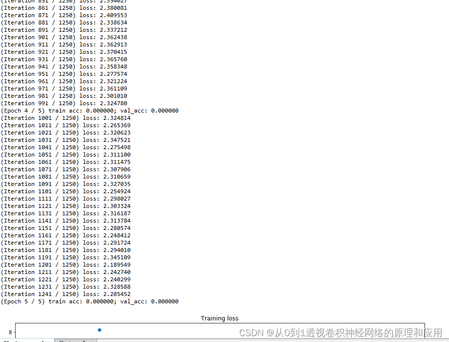
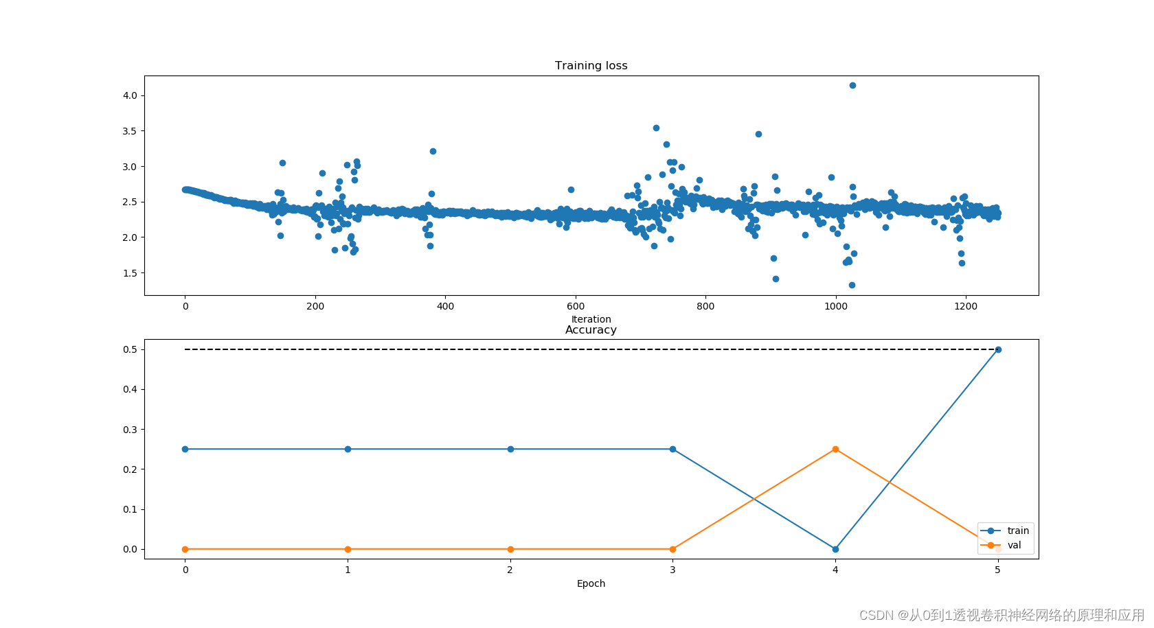
5.运行结果以及分析

这里选取500张图片作为训练样本，epoch = 5，batch = 2，每次随机选取2张图片，迭代 5 * 500/2 = 1250次，测试样本选取50张。

由运行结果可以看出，损失loss是逐步下降的。



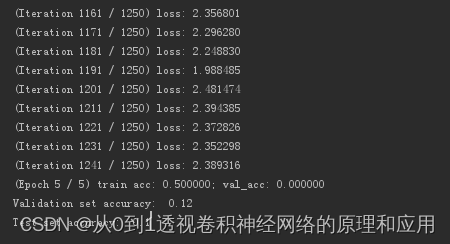
测试结果只有12%左右，原因有以下几点：

1. 模型比较简单，特征提取不能反映真实特征（一次卷积）；

2. 会出现过拟合问题；

3. 原始训练数据分类图片纹理复杂，这些图片可变性大，从而导致分类结果准确度低；

(airplane, automobile, bird, cat, deer, dog, frog, horse, ship, truck)

后续会通过tensorflow来实现CNN，测试准确率可以达到71.95%。

6. 参考文献

视觉一只白的博客《常用损失函数小结》https://blog.csdn.net/zhangjunp3/article/details/80467350

理想万岁的博客《Softmax函数详解与推导》：http://www.cnblogs.com/zongfa/p/8971213.html

下路派出所的博客《深度学习（九） 深度学习最全优化方法总结比较（SGD，Momentum，Nesterov Momentum，Adagrad，Adadelta，RMSprop，Adam）》

http://www.cnblogs.com/callyblog/p/8299074.html