


 本文是365天深度学习训练营的学习记录,探讨了不同优化器如Adam和SGD对模型训练的影响。作者使用VGG16模型并进行预处理,通过调整参数训练图像识别模型,对比了两种优化器在训练和验证阶段的精度与损失变化。
🍨 本文为🔗365天深度学习训练营 中的学习记录博客
🍦 参考文章:365天深度学习训练营-第11周:优化器对比实验(训练营内部成员可读)
🍖 原作者:K同学啊|接辅导、项目定制
🍺 本次主要是探究不同优化器、以及不同参数配置对模型的影响,结合训练营内部的文章[30分钟读懂优化器]目进行学习、研究。在论文当中我们也可以进行优化器的比对,以增加论文工作量。
🏡 运行环境:
电脑系统:Windows 10
语言环境:python 3.10
编译器:Pycharm 2022.1.1
深度学习环境:Pytorch
目录
一、前期准备
1.设置GPU
import tensorflow as tf
gpus = tf.config.list_physical_devices( "GPU" )
if gpus:
    gpu0 = gpus[0] #如果有多个GPU,仅使用第0个GPU
    tf.config.experimental.set_memory_growth(gpu0, True) #设置GPU显存用量按需使用
    tf.config.set_visible_devices([gpu0],"GPU" )
from tensorflow import keras
import matplotlib.pyplot as plt
import pandas as pd
import numpy as np
import warnings,os,PIL,pathlib

warnings.filterwarnings("ignore")
#忽略警告信息
plt.rcParams['font.sans-serif'] = [ 'SimHei'] # 用来正常显示中文标签
plt.rcParams['axes.unicode_minus'] = False
#用来正常显示负号
二、导入数据
1.导入数据
data_dir=r"D:/empire/48-data"
data_dir= pathlib.Path(data_dir)
image_count = len(list(data_dir.glob('*/*')))
print("图片总数为: ",image_count)
图片总数为: 1400
batch_size=16
img_height=336
img_width=336

train_ds = tf.keras.preprocessing.image_dataset_from_directory(

    data_dir,
    validation_split=0.2,
    subset= "training",
    seed=12,
    image_size=(img_height,img_width),
    batch_size=batch_size)

val_ds = tf.keras.preprocessing.image_dataset_from_directory(

    data_dir,
    validation_split=0.2,
    subset= "validation",
    seed=12,
    image_size=(img_height, img_width),
    batch_size=batch_size)

class_names = train_ds.class_names
print(class_names )
Found 1400 files belonging to 14 classes.
Using 1120 files for training.
Found 1400 files belonging to 14 classes.
Using 280 files for validation.
['Angelina Jolie', 'Brad Pitt', 'Denzel Washington', 'Hugh Jackman', 'Jennifer Lawrence', 'Johnny Depp', 'Kate Winslet', 'Leonardo DiCaprio', 'Natalie Portman', 'Nicole Kidman', 'Robert Downey Jr', 'Sandra Bullock', 'Tom Cruise', 'Will Smith']
2.检查数据
for image_batch,labels_batch in train_ds:
    print ( image_batch.shape )
    print(labels_batch.shape)
    break
(16, 336, 336, 3) (16,)
3.配置数据集
AUTOTUNE = tf.data.AUTOTUNE
def train_preprocessing( image,label):
    return ( image/255.0, label)
train_ds = (
    train_ds.cache()
    .shuffle(1000)
    .map(train_preprocessing)#这里可以设置预处理函数

#. batch(batch_ size)  #在image_ _dataset_ _from_ _directory处已经设置了batch_ size
    .prefetch( buffer_size=AUTOTUNE)
)
val_ds = (

    val_ds.cache()
    .shuffle( 1000)
    .map(train_preprocessing) #这里可以设置预处理函数
#   .batch(batch_ size)  #在image_ _dataset_ _from_ _directory处已经设置了batch_ size
    .prefetch( buffer_size=AUTOTUNE)
)
4.数据可视化
plt.figure(figsize=(10,8)) # 图形的宽为10高为5
plt.suptitle("数据展示")
for images,labels in train_ds.take(1):
    for i in range(15):
        plt.subplot(4,5,i + 1)
        plt.xticks([])
        plt.yticks([])
        plt.grid(False)
#显示图片
        plt.imshow( images[i])
#显示标签
        plt.xlabel(class_names[labels[i]-1])
        plt.show()
只能出来一列图片,不知道为啥!

三、构建模型
from tensorflow.keras.layers import Dropout,Dense,BatchNormalization
from tensorflow.keras.models import Model

def create_model (optimizer= 'adam'):

    #加载预训练模型
    vgg16_base_model = tf.keras.applications.vgg16.VGG16(weights= 'imagenet',
                                                                include_top=False,
                                                                input_shape=(img_width,img_height,3),
                                                                pooling= 'avg')


    for layer in vgg16_base_model.layers:
        layer.trainable=False


    x = vgg16_base_model.output

    x = Dense(170,activation='relu')(x)
    x = BatchNormalization()(x)
    x = Dropout(0.5)(x)
    output = Dense(len(class_names),activation='softmax')(x)
    vgg16_model = Model(inputs=vgg16_base_model.input,outputs=output)
    vgg16_model.compile(optimizer = optimizer,
                        loss= 'sparse_categorical_crossentropy',
                        metrics=['accuracy'])
    return vgg16_model
model1 = create_model(optimizer=tf.keras.optimizers.Adam())
model2 = create_model(optimizer=tf.keras.optimizers.SGD())
model2.summary()
Downloading data from https://storage.googleapis.com/tensorflow/keras-applications/vgg16/vgg16_weights_tf_dim_ordering_tf_kernels_notop.h5 58889256/58889256 [==============================] - 45s 1us/step Model: "model_1" _________________________________________________________________ Layer (type) Output Shape Param # ================================================================= input_2 (InputLayer) [(None, 336, 336, 3)] 0 block1_conv1 (Conv2D) (None, 336, 336, 64) 1792 block1_conv2 (Conv2D) (None, 336, 336, 64) 36928 block1_pool (MaxPooling2D) (None, 168, 168, 64) 0 block2_conv1 (Conv2D) (None, 168, 168, 128) 73856 block2_conv2 (Conv2D) (None, 168, 168, 128) 147584 block2_pool (MaxPooling2D) (None, 84, 84, 128) 0 block3_conv1 (Conv2D) (None, 84, 84, 256) 295168 block3_conv2 (Conv2D) (None, 84, 84, 256) 590080 block3_conv3 (Conv2D) (None, 84, 84, 256) 590080 block3_pool (MaxPooling2D) (None, 42, 42, 256) 0 block4_conv1 (Conv2D) (None, 42, 42, 512) 1180160 block4_conv2 (Conv2D) (None, 42, 42, 512) 2359808 block4_conv3 (Conv2D) (None, 42, 42, 512) 2359808 block4_pool (MaxPooling2D) (None, 21, 21, 512) 0 block5_conv1 (Conv2D) (None, 21, 21, 512) 2359808 block5_conv2 (Conv2D) (None, 21, 21, 512) 2359808 block5_conv3 (Conv2D) (None, 21, 21, 512) 2359808 block5_pool (MaxPooling2D) (None, 10, 10, 512) 0 global_average_pooling2d_1 (None, 512) 0 (GlobalAveragePooling2D) dense_2 (Dense) (None, 170) 87210 batch_normalization_1 (Batc (None, 170) 680 hNormalization) dropout_1 (Dropout) (None, 170) 0 dense_3 (Dense) (None, 14) 2394 ================================================================= Total params: 14,804,972 Trainable params: 89,944 Non-trainable params: 14,715,028 _________________________________________________________________
四、训练模型
NO_EPOCHS = 5
history_model1 = model1.fit(train_ds,epochs=NO_EPOCHS,verbose=1,validation_data=val_ds )
history_model2 = model2.fit(train_ds,epochs=NO_EPOCHS,verbose=1,validation_data=val_ds )
Epoch 1/5
70/70 [==============================] - 396s 5s/step - loss: 2.6283 - accuracy: 0.1946 - val_loss: 2.5711 - val_accuracy: 0.0929
Epoch 2/5
70/70 [==============================] - 374s 5s/step - loss: 1.9258 - accuracy: 0.3598 - val_loss: 2.3922 - val_accuracy: 0.2107
Epoch 3/5
70/70 [==============================] - 373s 5s/step - loss: 1.6430 - accuracy: 0.4732 - val_loss: 2.2054 - val_accuracy: 0.3000
Epoch 4/5
70/70 [==============================] - 374s 5s/step - loss: 1.4522 - accuracy: 0.5268 - val_loss: 2.0061 - val_accuracy: 0.4071
Epoch 5/5
70/70 [==============================] - 374s 5s/step - loss: 1.2903 - accuracy: 0.5589 - val_loss: 1.8623 - val_accuracy: 0.3429
Epoch 1/5
70/70 [==============================] - 374s 5s/step - loss: 2.8286 - accuracy: 0.1286 - val_loss: 2.6562 - val_accuracy: 0.0821
Epoch 2/5
70/70 [==============================] - 373s 5s/step - loss: 2.3253 - accuracy: 0.2393 - val_loss: 2.5055 - val_accuracy: 0.1321
Epoch 3/5
70/70 [==============================] - 373s 5s/step - loss: 2.0961 - accuracy: 0.3125 - val_loss: 2.3748 - val_accuracy: 0.2393
Epoch 4/5
70/70 [==============================] - 374s 5s/step - loss: 1.9022 - accuracy: 0.3670 - val_loss: 2.2156 - val_accuracy: 0.3214
Epoch 5/5
70/70 [==============================] - 373s 5s/step - loss: 1.8107 - accuracy: 0.3946 - val_loss: 2.1071 - val_accuracy: 0.3250
五、评估模型
1.Accuracy与Loss图
from matplotlib.ticker import MultipleLocator
plt.rcParams['savefig.dpi']=300
plt.rcParams['figure.dpi']=300

acc1=history_model1.history['accuracy']
acc2=history_model2.history['accuracy']
val_acc1=history_model1.history['val_accuracy']
val_acc2=history_model2.history['val_accuracy']

loss1=history_model1.history['loss']
loss2=history_model2.history['loss']
val_loss1=history_model1.history['val_loss']
val_loss2=history_model2.history['val_loss']

epochs_range=range(len(acc1))

plt.figure(figsize=(16,4))
plt.subplot(1,2,1)

plt.plot(epochs_range,acc1,label='Training Accuracy-Adam')
plt.plot(epochs_range,acc2,label='Training Accuracy-SGD')
plt.plot(epochs_range,val_acc1,label='Validation Accuracy-Adam')
plt.plot(epochs_range,val_acc2,label='Validation Accuracy-SGD')
plt.legend(loc='lower right')
plt.title('Training and Validation Accuracy')

ax=plt.gca()
ax.xaxis.set_major_locator(MultipleLocator(1))

plt.subplot(1,2,2)
plt.plot(epochs_range,loss1,label='Training Loss-Adam')
plt.plot(epochs_range,loss2,label='Training Loss-SGD')
plt.plot(epochs_range,val_loss1,label='Validation Loss-Adam')
plt.plot(epochs_range,val_loss2,label='Validation Loss-SGD')
plt.legend(loc='upper right')
plt.title('Training and Validation Loss')


ax=plt.gca()
ax.xaxis.set_major_locator(MultipleLocator(1))

plt.show() 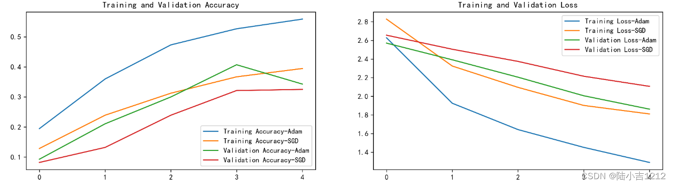
2.模型评估
def test_accuracy_report(model):
    score=model.evaluate(val_ds,verbose=0)
    print('Loss function:%s,accuracy:' % score[0],score[1])

test_accuracy_report(model2)
oss function:2.107053518295288,accuracy: 0.32499998807907104


 被折叠的 条评论
为什么被折叠?
被折叠的 条评论
为什么被折叠?
 到【灌水乐园】发言


