利用 PINN 解热传导方程的原理与实现

m0_68330627

已于 2024-11-09 22:38:26 修改

阅读量4k

点赞数 46

文章标签： python 神经网络

于 2024-11-09 22:37:43 首次发布

本文链接：https://blog.csdn.net/m0_68330627/article/details/143652512

版权

引言

传统的数值方法，如有限差分、有限元等，已经被广泛用于求解偏微分方程（PDEs）。然而，它们在高维问题或复杂几何形状下计算成本高昂。近年来，物理信息神经网络（Physics-Informed Neural Networks，PINNs）作为一种新兴的数值方法，利用深度学习的强大表示能力和自动微分机制，可以有效地求解 PDEs。

本文将基于给定的代码，详细介绍 PINN 如何用于求解一维热传导方程，并给出必要的公式推导。我们还将对代码进行适当的修改，以更好地理解和实现这一过程。

一维热传导方程

一维热传导方程描述了温度在一维空间中的传播，其基本形式为：

$\frac{\partial u}{\partial t} = \alpha \frac{\partial^2 u}{\partial x^2}$

其中，( u(x, t) ) 表示位置 ( x ) 在时间 ( t ) 时的温度分布，( \alpha ) 是热扩散系数。

初始条件和边界条件

为使问题确定，我们需要给定初始条件和边界条件：

初始条件（时间 ( t=0 )）：
$u (x, 0) = f (x)$
边界条件（空间 ( x=a ) 和 ( x=b )）：
$g_1(t), \quad u(b, t) = g_2(t)$

PINN 的基本原理

PINN 的核心思想是将 PDE、初始条件、边界条件嵌入到神经网络的损失函数中，通过最小化损失函数，使神经网络的输出满足给定的物理方程和条件。

损失函数的构建

对热传导方程，我们的损失函数包括三部分：

物理损失（PDE 损失）：确保网络的输出满足热传导方程。
$\mathcal{L}_{\text{PDE}} = \left\| \frac{\partial u}{\partial t} - \alpha \frac{\partial^2 u}{\partial x^2} \right\|^2$
初始条件损失：确保网络的输出在初始时刻满足初始条件。
$\mathcal{L}_{\text{IC}} = \left\| u(x, 0) - f(x) \right\|^2$
边界条件损失：确保网络的输出在边界处满足边界条件。
$\mathcal{L}_{\text{BC}} = \left\| u(a, t) - g_1(t) \right\|^2 + \left\| u(b, t) - g_2(t) \right\|^2$

总的损失函数为：
$\mathcal{L} = \mathcal{L}_{\text{PDE}} + \mathcal{L}_{\text{IC}} + \mathcal{L}_{\text{BC}}$

自动微分机制

利用深度学习框架（如 PyTorch）的自动微分，我们可以方便地计算输出关于输入的导数，这对于计算 PDE 中的偏导数非常方便。

代码实现与解读

下面我们将对给定的代码进行解读，并适当修改以求解热传导方程。

导入必要的库

import torch
import torch.nn as nn
import matplotlib.pyplot as plt
import numpy as np
from tqdm import tqdm

# 判断是否有可用的 GPU
device = torch.device("cuda" if torch.cuda.is_available() else "cpu")
print(f"Using device: {device}")

定义神经网络架构

神经网络接收 ( (t, x) ) 作为输入，输出对应的 ( u(t, x) )。

# 定义网络结构
class PINN(nn.Module):
    def __init__(self):
        super(PINN, self).__init__()
        self.layer = nn.Sequential(
            nn.Linear(2, 20), nn.Tanh(),
            nn.Linear(20, 20), nn.Tanh(),
            nn.Linear(20, 20), nn.Tanh(),
            nn.Linear(20, 20), nn.Tanh(),
            nn.Linear(20, 20), nn.Tanh(),
            nn.Linear(20, 1)
        ).to(device)
    
    def forward(self, t, x):
        u = self.layer(torch.cat([t, x], dim=1))
        return u

修改说明：将隐藏层的神经元数量从 16 调整为 20，以增强网络的表示能力。

定义损失函数

物理损失（PDE 损失）

# 定义热传导方程中的物理损失
def physics_loss(model, t, x, alpha=0.5):
    u = model(t, x)
    u_t = torch.autograd.grad(u, t, torch.ones_like(u), create_graph=True)[0]
    u_x = torch.autograd.grad(u, x, torch.ones_like(u), create_graph=True)[0]
    u_xx = torch.autograd.grad(u_x, x, torch.ones_like(u), create_graph=True)[0]
    f = (u_t - alpha * u_xx).pow(2).mean()
    return f

修改说明：修正 torch.ones_like 的输入，确保形状匹配。同时，将热扩散系数 ( \alpha ) 设为可调参数。

边界条件损失

# 定义边界条件损失
def boundary_loss(model, t_bc, x_left, x_right):
    u_left = model(t_bc, x_left)
    u_right = model(t_bc, x_right)
    loss_left = (u_left - g1(t_bc)).pow(2).mean()
    loss_right = (u_right - g2(t_bc)).pow(2).mean()
    return loss_left + loss_right

# 定义边界条件函数
def g1(t):
    return torch.zeros_like(t)

def g2(t):
    return torch.zeros_like(t)

修改说明：将边界条件设为 ( u(-1, t) = 0 ) 和 ( u(1, t) = 0 )，对应于固定温度的边界条件。

初始条件损失

# 初始条件损失
def initial_loss(model, x_ic):
    t_0 = torch.zeros_like(x_ic).to(device)
    u_init = model(t_0, x_ic)
    u_exact = f(x_ic)
    return (u_init - u_exact).pow(2).mean()

# 定义初始条件函数
def f(x):
    return torch.sin(np.pi * x)

修改说明：将初始条件设为 ( u(x, 0) = \sin(\pi x) )。

训练过程

# 训练模型并记录损失
def train(model, optimizer, num_epochs):
    losses = []
    model.to(device)
    for epoch in tqdm(range(num_epochs), desc="Training"):
        optimizer.zero_grad()

        # 随机采样 t 和 x，并确保 requires_grad=True
        t = torch.rand(3000, 1).to(device)
        x = torch.rand(3000, 1).to(device) * 2 - 1  # x ∈ [-1, 1]
        t.requires_grad = True
        x.requires_grad = True

        # 物理损失
        f_loss = physics_loss(model, t, x)

        # 边界条件损失
        t_bc = torch.rand(500, 1).to(device)
        x_left = -torch.ones(500, 1).to(device)
        x_right = torch.ones(500, 1).to(device)
        bc_loss = boundary_loss(model, t_bc, x_left, x_right)

        # 初始条件损失
        x_ic = torch.rand(1000, 1).to(device) * 2 - 1
        ic_loss = initial_loss(model, x_ic)

        # 总损失
        loss = f_loss + bc_loss + ic_loss
        loss.backward()
        optimizer.step()

        # 记录损失
        losses.append(loss.item())

        if epoch % 1000 == 0:
            print(f'Epoch {epoch}, Loss: {loss.item()}')
     
    return losses

初始化模型和优化器

# 初始化模型和优化器
model = PINN()
optimizer = torch.optim.Adam(model.parameters(), lr=1e-3)

训练模型

# 训练模型
losses = train(model, optimizer, num_epochs=10000)

结果展示

绘制训练损失曲线

# 绘制损失曲线
def plot_loss(losses):
    plt.figure(figsize=(8, 5))
    plt.plot(losses, color='blue', lw=2)
    plt.xlabel('Epoch', fontsize=14)
    plt.ylabel('Loss', fontsize=14)
    plt.title('Training Loss Curve', fontsize=16)
    plt.grid(True)
    plt.tight_layout()
    plt.show()

plot_loss(losses)

绘制解的图像

# 绘制数值解图像
def plot_solution(model):
    x = torch.linspace(-1, 1, 100).unsqueeze(1).to(device)
    t = torch.full((100, 1), 0.0).to(device)  # 在 t=0 时绘制解
    with torch.no_grad():
        u_pred = model(t, x).cpu().numpy()
    
    # 参考解 u(0,x) = sin(πx)
    u_exact = np.sin(np.pi * x.cpu().numpy())
    
    plt.figure(figsize=(8, 5))
    plt.plot(x.cpu().numpy(), u_pred, label='Predicted Solution', color='red', lw=2)
    plt.plot(x.cpu().numpy(), u_exact, label='Exact Solution (Initial)', color='blue', lw=2, linestyle='dashed')
    plt.xlabel('x', fontsize=14)
    plt.ylabel('u(t=0, x)', fontsize=14)
    plt.title('Heat Conduction Equation Solution at t=0', fontsize=16)
    plt.legend(fontsize=12)
    plt.grid(True)
    plt.tight_layout()
    plt.show()

plot_solution(model)

在这里插入图片描述

绘制三维曲面图

# 绘制整个 (x, t) 平面的解
def plot_solution_3d(model):
    # 创建 (x, t) 网格
    x = torch.linspace(-1, 1, 100).unsqueeze(1).to(device)
    t = torch.linspace(0, 1, 100).unsqueeze(1).to(device)
    X, T = torch.meshgrid(x.squeeze(), t.squeeze(), indexing='ij')
    
    # 将 X 和 T 拉平，方便模型预测
    x_flat = X.reshape(-1, 1).to(device)
    t_flat = T.reshape(-1, 1).to(device)

    with torch.no_grad():
        u_pred = model(t_flat, x_flat).cpu().numpy().reshape(100, 100)

    # 绘制三维曲面图
    fig = plt.figure(figsize=(10, 7))
    ax = fig.add_subplot(111, projection='3d')
    ax.plot_surface(X.cpu().numpy(), T.cpu().numpy(), u_pred, cmap='viridis')

    ax.set_xlabel('x', fontsize=12)
    ax.set_ylabel('t', fontsize=12)
    ax.set_zlabel('u(t, x)', fontsize=12)
    ax.set_title('Solution of Heat Conduction Equation on (x, t) Plane', fontsize=14)
    plt.show()

plot_solution_3d(model)   # 三维曲面图

在这里插入图片描述

绘制二维等高线图

# 绘制二维等高线图
def plot_solution_contour(model):
    # 创建 (x, t) 网格
    x = torch.linspace(-1, 1, 100).unsqueeze(1).to(device)
    t = torch.linspace(0, 1, 100).unsqueeze(1).to(device)
    X, T = torch.meshgrid(x.squeeze(), t.squeeze(), indexing='ij')

    # 将 X 和 T 拉平，方便模型预测
    x_flat = X.reshape(-1, 1).to(device)
    t_flat = T.reshape(-1, 1).to(device)

    with torch.no_grad():
        u_pred = model(t_flat, x_flat).cpu().numpy().reshape(100, 100)

    # 绘制二维等高线图
    plt.figure(figsize=(8, 6))
    plt.contourf(X.cpu().numpy(), T.cpu().numpy(), u_pred, 100, cmap='viridis')
    plt.colorbar(label='u(t, x)')
    
    plt.xlabel('x', fontsize=12)
    plt.ylabel('t', fontsize=12)
    plt.title('Heat Conduction Equation Solution', fontsize=14)
    
    plt.tight_layout()
    plt.show()
    
plot_solution_contour(model)   # 二维等高线图

在这里插入图片描述

解释与分析

初始条件的验证

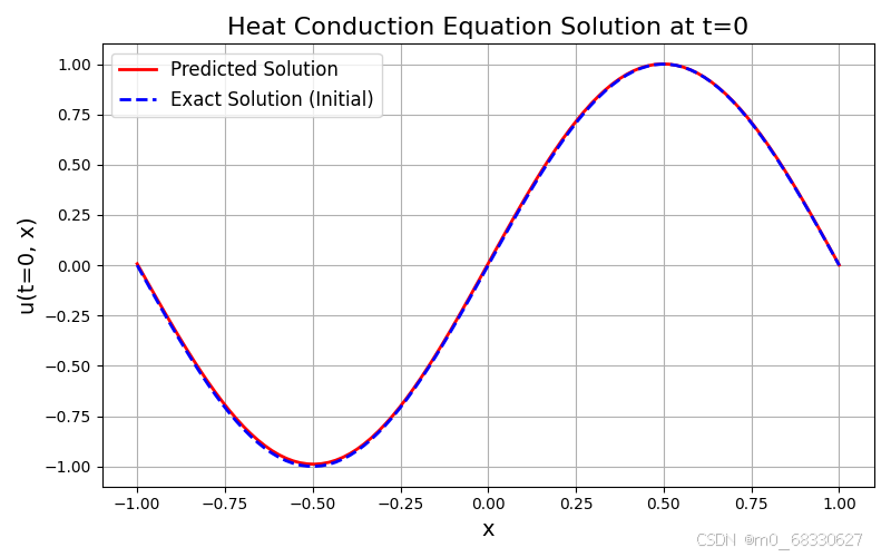
从初始条件的图像可以看出，模型在 ( t=0 ) 时刻的预测与初始条件 ( u(x, 0) = \sin(\pi x) ) 基本吻合，说明模型成功学习到了初始状态。

整体解的展示

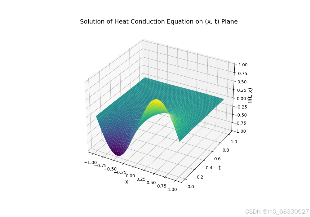
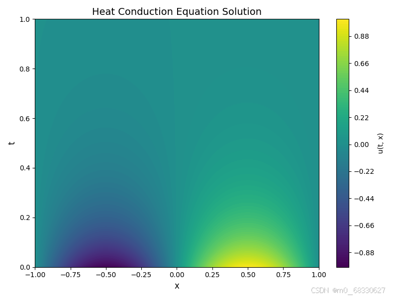
通过三维曲面图和二维等高线图，我们可以观察到热传导方程解随时间和空间的变化。随着时间的推移，温度逐渐趋于稳定，这是热传导方程的典型特征。

结论

本文详细介绍了如何利用 PINN 求解一维热传导方程。通过将 PDE、初始条件和边界条件嵌入到神经网络的损失函数中，我们可以训练模型使其输出满足所需的物理条件。实验结果表明，PINN 能够有效地逼近热传导方程的解，为数值求解 PDE 提供了一种新颖且高效的途径。

参考文献

Raissi, M., Perdikaris, P., & Karniadakis, G. E. (2019). Physics-informed neural networks: A deep learning framework for solving forward and inverse problems involving nonlinear partial differential equations. Journal of Computational Physics, 378, 686-707.

完整代码

import torch
import torch.nn as nn
import matplotlib.pyplot as plt
import numpy as np
from tqdm import tqdm

# 判断是否有可用的 GPU
device = torch.device("cuda" if torch.cuda.is_available() else "cpu")
print(f"Using device: {device}")

class PINN(nn.Module):
    def __init__(self):
        super(PINN, self).__init__()
        self.layer = nn.Sequential(
            nn.Linear(2, 20), nn.Tanh(),
            nn.Linear(20, 20), nn.Tanh(),
            nn.Linear(20, 20), nn.Tanh(),
            nn.Linear(20, 20), nn.Tanh(),
            nn.Linear(20, 20), nn.Tanh(),
            nn.Linear(20, 1)
        ).to(device)
    
    def forward(self, t, x):
        u = self.layer(torch.cat([t, x], dim=1))
        return u
    
def physics_loss(model, t, x, alpha=0.5):
    u = model(t, x)
    u_t = torch.autograd.grad(u, t, torch.ones_like(u), create_graph=True)[0]
    u_x = torch.autograd.grad(u, x, torch.ones_like(u), create_graph=True)[0]
    u_xx = torch.autograd.grad(u_x, x, torch.ones_like(u), create_graph=True)[0]
    f = (u_t - alpha * u_xx).pow(2).mean()
    return f

def boundary_loss(model, t_bc, x_left, x_right):
    u_left = model(t_bc, x_left)
    u_right = model(t_bc, x_right)
    loss_left = (u_left - g1(t_bc)).pow(2).mean()
    loss_right = (u_right - g2(t_bc)).pow(2).mean()
    return loss_left + loss_right

# 定义边界条件函数
def g1(t):
    return torch.zeros_like(t)

def g2(t):
    return torch.zeros_like(t)

def initial_loss(model, x_ic):
    t_0 = torch.zeros_like(x_ic).to(device)
    u_init = model(t_0, x_ic)
    u_exact = f(x_ic)
    return (u_init - u_exact).pow(2).mean()

def f(x):
    return torch.sin(np.pi * x)

def train(model, optimizer, num_epochs):
    losses = []
    model.to(device)
    for epoch in tqdm(range(num_epochs), desc="Training"):
        optimizer.zero_grad()

        # 随机采样 t 和 x，并确保 requires_grad=True
        t = torch.rand(3000, 1).to(device)
        x = torch.rand(3000, 1).to(device) * 2 - 1  # x ∈ [-1, 1]
        t.requires_grad = True
        x.requires_grad = True

        # 物理损失
        f_loss = physics_loss(model, t, x)

        # 边界条件损失
        t_bc = torch.rand(500, 1).to(device)
        x_left = -torch.ones(500, 1).to(device)
        x_right = torch.ones(500, 1).to(device)
        bc_loss = boundary_loss(model, t_bc, x_left, x_right)

        # 初始条件损失
        x_ic = torch.rand(1000, 1).to(device) * 2 - 1
        ic_loss = initial_loss(model, x_ic)

        # 总损失
        loss = f_loss + bc_loss + ic_loss
        loss.backward()
        optimizer.step()

        # 记录损失
        losses.append(loss.item())

        if epoch % 1000 == 0:
            print(f'Epoch {epoch}, Loss: {loss.item()}')
     
    return losses

model = PINN()
optimizer = torch.optim.Adam(model.parameters(), lr=1e-3)

losses = train(model, optimizer, num_epochs=10000)

def plot_loss(losses):
    plt.figure(figsize=(8, 5))
    plt.plot(losses, color='blue', lw=2)
    plt.xlabel('Epoch', fontsize=14)
    plt.ylabel('Loss', fontsize=14)
    plt.title('Training Loss Curve', fontsize=16)
    plt.grid(True)
    plt.tight_layout()
    plt.show()

plot_loss(losses)

def plot_solution(model):
    x = torch.linspace(-1, 1, 100).unsqueeze(1).to(device)
    t = torch.full((100, 1), 0.0).to(device)  # 在 t=0 时绘制解
    with torch.no_grad():
        u_pred = model(t, x).cpu().numpy()
    
    # 参考解 u(0,x) = sin(πx)
    u_exact = np.sin(np.pi * x.cpu().numpy())
    
    plt.figure(figsize=(8, 5))
    plt.plot(x.cpu().numpy(), u_pred, label='Predicted Solution', color='red', lw=2)
    plt.plot(x.cpu().numpy(), u_exact, label='Exact Solution (Initial)', color='blue', lw=2, linestyle='dashed')
    plt.xlabel('x', fontsize=14)
    plt.ylabel('u(t=0, x)', fontsize=14)
    plt.title('Heat Conduction Equation Solution at t=0', fontsize=16)
    plt.legend(fontsize=12)
    plt.grid(True)
    plt.tight_layout()
    plt.savefig('pinn1.png')
    plt.show()

plot_solution(model)

def plot_solution_3d(model):
    # 创建 (x, t) 网格
    x = torch.linspace(-1, 1, 100).unsqueeze(1).to(device)
    t = torch.linspace(0, 1, 100).unsqueeze(1).to(device)
    X, T = torch.meshgrid(x.squeeze(), t.squeeze(), indexing='ij')
    
    # 将 X 和 T 拉平，方便模型预测
    x_flat = X.reshape(-1, 1).to(device)
    t_flat = T.reshape(-1, 1).to(device)

    with torch.no_grad():
        u_pred = model(t_flat, x_flat).cpu().numpy().reshape(100, 100)

    # 绘制三维曲面图
    fig = plt.figure(figsize=(10, 7))
    ax = fig.add_subplot(111, projection='3d')
    ax.plot_surface(X.cpu().numpy(), T.cpu().numpy(), u_pred, cmap='viridis')

    ax.set_xlabel('x', fontsize=12)
    ax.set_ylabel('t', fontsize=12)
    ax.set_zlabel('u(t, x)', fontsize=12)
    ax.set_title('Solution of Heat Conduction Equation on (x, t) Plane', fontsize=14)
    plt.savefig('pinn3.png')
    plt.show()

plot_solution_3d(model)   # 三维曲面图

def plot_solution_contour(model):
    # 创建 (x, t) 网格
    x = torch.linspace(-1, 1, 100).unsqueeze(1).to(device)
    t = torch.linspace(0, 1, 100).unsqueeze(1).to(device)
    X, T = torch.meshgrid(x.squeeze(), t.squeeze(), indexing='ij')

    # 将 X 和 T 拉平，方便模型预测
    x_flat = X.reshape(-1, 1).to(device)
    t_flat = T.reshape(-1, 1).to(device)

    with torch.no_grad():
        u_pred = model(t_flat, x_flat).cpu().numpy().reshape(100, 100)

    # 绘制二维等高线图
    plt.figure(figsize=(8, 6))
    plt.contourf(X.cpu().numpy(), T.cpu().numpy(), u_pred, 100, cmap='viridis')
    plt.colorbar(label='u(t, x)')
    
    plt.xlabel('x', fontsize=12)
    plt.ylabel('t', fontsize=12)
    plt.title('Heat Conduction Equation Solution', fontsize=14)
    
    plt.tight_layout()
    plt.savefig('pinn2.png')
    plt.show()
    
plot_solution_contour(model)  
ape(-1, 1).to(device)

    with torch.no_grad():
        u_pred = model(t_flat, x_flat).cpu().numpy().reshape(100, 100)

    # 绘制二维等高线图
    plt.figure(figsize=(8, 6))
    plt.contourf(X.cpu().numpy(), T.cpu().numpy(), u_pred, 100, cmap='viridis')
    plt.colorbar(label='u(t, x)')
    
    plt.xlabel('x', fontsize=12)
    plt.ylabel('t', fontsize=12)
    plt.title('Heat Conduction Equation Solution', fontsize=14)
    
    plt.tight_layout()
    plt.savefig('pinn2.png')
    plt.show()
    
plot_solution_contour(model)