python画WRF垂直剖面

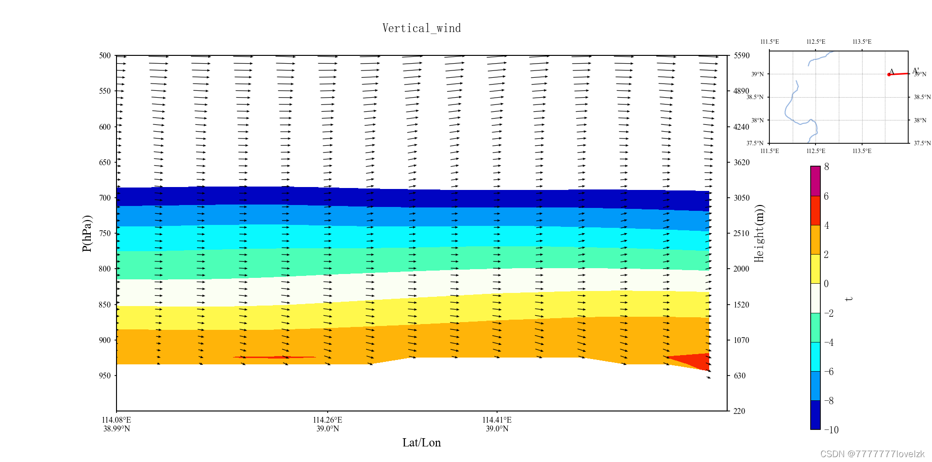
一直很想画垂直剖面图，借鉴了很多大佬的笔记，包括NCL和GrADS代码，最后发现还是python好用，然后自己根据需要改了改，此贴更多为自己记录学习下~废话不多说，附上代码。（图为T2例图，可以根据需要换参数)

import netCDF4 as nc
from wrf import to_np,getvar,CoordPair,vertcross,interplevel
import cartopy.crs as ccrs
from cartopy.io import shapereader
filename =shapereader.natural_earth()
import cartopy.feature as cfeat
import matplotlib.pyplot as plt
import cmaps
import matplotlib as mpl
import matplotlib.ticker as mticker
from cartopy.mpl.ticker import LongitudeFormatter, LatitudeFormatter
from matplotlib.font_manager import FontProperties
import numpy as np

Simsun = FontProperties(fname="E:\\anaconda\\Lib\\site-packages\\matplotlib\\times.ttf")
Times = FontProperties(fname="E:\\anaconda\\Lib\\site-packages\\matplotlib\\times.ttf")
mpl.rcParams['axes.unicode_minus']=False
config = {
    "font.family":'serif',
    "mathtext.fontset": 'stix',
    "font.serif": ['SimSun'],
}
mpl.rcParams.update(config)

big_p,small_p,interval_p=1000,500,50
start_lon,end_lon,interval_lon=114.1,114.6,0.2
start_lat,end_lat=38.98,39.01
startpoint = CoordPair(lat=start_lat, lon=start_lon)
endpoint = CoordPair(lat=end_lat, lon=end_lon)
ncfile=nc.Dataset('E:\wrf 20211209 hysplit\wrfoutd03.00')
t=getvar(ncfile,'tc',timeidx=48)
lat=getvar(ncfile,'lat')
lon=getvar(ncfile,'lon')
height=getvar(ncfile,'height')
hgt=getvar(ncfile,'HGT')
height2earth=height-hgt
ua=getvar(ncfile,'ua',timeidx=48)
va=getvar(ncfile,'va',timeidx=48)
wa=getvar(ncfile,'wa',timeidx=48)
wa = wa * 10
p = getvar(ncfile, 'pressure', timeidx=48)
t_vert = vertcross(t, p, wrfin=ncfile, start_point=startpoint, end_point=endpoint, latlon=True)
ua_vert = vertcross(ua, p, wrfin=ncfile, start_point=startpoint, end_point=endpoint, latlon=True)
va_vert = vertcross(va, p, wrfin=ncfile, start_point=startpoint, end_point=endpoint, latlon=True)
wa_vert = vertcross(wa, p, wrfin=ncfile, start_point=startpoint, end_point=endpoint, latlon=True)
ws_vert = np.sqrt(ua_vert ** 2 + va_vert ** 2)
wdir_vert = np.arctan2(va_vert, ua_vert) * 180 / np.pi
line_angel = np.arctan2(end_lat - start_lat, end_lon - start_lon) * 180 / np.pi
vl_angel = wdir_vert - line_angel
vl_angel = np.cos(np.deg2rad(vl_angel))
ws_vert = ws_vert * vl_angel

lonlist, latlist, hlist = [], [], []
plist = to_np(va_vert.coords['vertical'])
for i in range(len(ua_vert.coords['xy_loc'])):
    s = str(ua_vert.coords['xy_loc'][i].values)
    lonlist.append(float(s[s.find('lon=') + 4:s.find('lon=') + 12]))
    latlist.append(float(s[s.find('lat=') + 4:s.find('lat=') + 12]))
for i in range(big_p, small_p - interval_p, -interval_p):
    hlist.append(float(np.max(interplevel(height2earth, p, i)).values))
hlist = np.array([int(i) for i in hlist])
str_lonlist, float_lonlist = [], []
a = np.mgrid[0:len(lonlist) - 1:complex(str(int(round((end_lon + interval_lon - start_lon) / interval_lon))) + 'j')]
a = np.around(a, decimals=0)
for i in range(int((end_lon + interval_lon - start_lon) / interval_lon)):
    float_lonlist.append(lonlist[int(a[i])])
    lo, la = round(lonlist[int(a[i])], 2), round(latlist[int(a[i])], 2)
    str_lonlist.append(str(lo) + '°E' + "\n" + str(la) + '°N')

fig=plt.figure(figsize=(10,10),dpi=150)
axe=plt.subplot(1,1,1)
axe.set_title('Vertical_wind',fontsize=12,y=1.05)
axe.set_xlim(start_lon, end_lon)
axe.set_ylim(small_p, big_p)
axe.invert_yaxis()  # 翻转纵坐标
axe.grid(color='gray', linestyle=':', linewidth=0.7, axis='y')
plt.xticks(float_lonlist, str_lonlist, fontsize=8, color='k')
axe.set_xlabel('Lat/Lon', fontproperties=Simsun, fontsize=12)
axe.get_xaxis().set_visible('True')
plt.yticks(fontsize=8, color='k')
axe.get_yaxis().set_visible('True')
axe.set_yticks(np.arange(small_p, big_p, interval_p))
axe.set_ylabel('P$\mathrm{(hPa))}$', fontproperties=Simsun, fontsize=12)
axe.tick_params(length=2)
labels = axe.get_xticklabels() + axe.get_yticklabels()
[label.set_fontproperties(FontProperties(fname="E:\\anaconda\\Lib\\site-packages\\matplotlib\\times.ttf", size=8)) for label in labels]

axe.grid(color='gray', linestyle=":", linewidth=0.7, axis='y')

t_level=np.arange(-10,10,2)
contourf = axe.contourf(lonlist, plist, t_vert, levels=t_level, cmap=cmaps.NCV_jaisnd,extend='neither')
axe.quiver(lonlist, plist, ws_vert, wa_vert, pivot='mid',
           width=0.001, scale=700, color='k', headwidth=4,
           alpha=1)

fig.subplots_adjust(right=0.78)
rect = [0.87, 0.07, 0.01, 0.57]
cbar_ax = fig.add_axes(rect)
cb = fig.colorbar(contourf, drawedges=True, ticks=t_level, cax=cbar_ax, orientation='vertical',spacing='uniform')
cb.set_label('t', fontsize=12)
cb.ax.tick_params(length=0)
# labels = cb.ax.get_xticklabels()+cb.ax.get_yticklabels()
# [label.set_fontproperties(FontProperties(fname="E:\\anaconda\\Lib\\site-packages\\matplotlib\\times.ttf",size=10)) for label in labels]

axe1 = fig.add_axes([0.8,0.69,0.2,0.2], projection=ccrs.PlateCarree())
LAKES_border=cfeat.NaturalEarthFeature('physical','lakes','10m',edgecolor='black',facecolor='never')
axe1.add_feature(cfeat.COASTLINE.with_scale("10m"), linewidth=0.7, color='k')
axe1.add_feature(cfeat.RIVERS.with_scale("10m"))
axe1.add_feature(cfeat.OCEAN.with_scale("10m"))
axe1.add_feature(cfeat.LAKES.with_scale("10m"))
axe1.set_extent([111.5, 114.5, 37.5, 39.5], crs=ccrs.PlateCarree())
gl = axe1.gridlines(crs=ccrs.PlateCarree(), draw_labels=False, linewidth=0.5, color='gray',linestyle=':')
gl.xlocator = mticker.FixedLocator(np.arange(111.5, 114.5, 0.5))
gl.ylocator = mticker.FixedLocator(np.arange(37.5, 39.5, 0.5))
gl.xformatter = LongitudeFormatter
gl.yformatter = LatitudeFormatter
axe1.set_xticks(np.arange(111.5, 114.5, 1), crs=ccrs.PlateCarree())
axe1.set_yticks(np.arange(37.5, 39.5, 0.5), crs=ccrs.PlateCarree())
plt.tick_params(top=True,bottom=True,left=True,right=True)
plt.tick_params(labeltop=True,labelleft=True,labelright=True,labelbottom=True)
axe1.xaxis.set_major_formatter(LongitudeFormatter())
axe1.yaxis.set_major_formatter(LatitudeFormatter())
axe1.set_xticks(np.arange(111.5, 114.5, 1), crs=ccrs.PlateCarree(), minor=True)
axe1.set_yticks(np.arange(37.5, 39.5, 0.5), crs=ccrs.PlateCarree(), minor=True)
axe1.tick_params(labelcolor='k',length=2)
labels = axe1.get_xticklabels() + axe1.get_yticklabels()
[label.set_fontproperties(FontProperties(fname="E:\\anaconda\\Lib\\site-packages\\matplotlib\\times.ttf",size=6)) for label in labels]


axe1.plot([lonlist[0], lonlist[-1]], [latlist[0], latlist[-1]], color='red', linewidth=1.5,linestyle='-')
axe1.plot(lonlist[0], latlist[0], marker='o', color='red', markersize=2.5)
axe1.plot(lonlist[-1], latlist[-1], marker='o', color='red', markersize=2.5)
axe1.text(lonlist[0], latlist[0], 'A', fontproperties=FontProperties(fname="E:\\anaconda\\Lib\\site-packages\\matplotlib\\times.ttf", size=8))
axe1.text(lonlist[-1], latlist[-1], 'A'+"'", fontproperties=FontProperties(fname="E:\\anaconda\\Lib\\site-packages\\matplotlib\\times.ttf", size=8))

axe_sub = axe.twinx()
axe_sub.set_ylim(hlist[0],hlist[-1])
axe_sub.set_yticks(np.mgrid[hlist[0]:hlist[-1]:complex(str(int(hlist.shape[0])) + 'j')])
round_hlist=np.around(hlist,-1)
axe_sub.set_yticklabels(round_hlist)
axe_sub.set_ylabel('Height$\mathrm{(m))}$', fontsize=12)
axe_sub.tick_params(labelcolor='black', length=3)
labels = axe_sub.get_xticklabels() + axe_sub.get_yticklabels()
[label.set_fontproperties(FontProperties(fname="E:\\anaconda\\Lib\\site-packages\\matplotlib\\times.ttf", size=8)) for label in labels]

plt.show()