


LBP指局部二值模式,英文全称:Local Binary Pattern,是一种用来描述图像局部特征的算子,LBP特征具有灰度不变性和旋转不变性等显著优点。它是由T. Ojala, M.Pietikäinen, 和 D. Harwood [1][2]在1994年提出,由于LBP特征计算简单、效果较好,因此LBP特征在计算机视觉的许多领域都得到了广泛的应用,LBP特征比较出名的应用是用在人脸识别和目标检测中,在计算机视觉开源库Opencv中有使用LBP特征进行人脸识别的接口,也有用LBP特征训练目标检测分类器的方法,Opencv实现了LBP特征的计算,但没有提供一个单独的计算LBP特征的接口。
二、LBP特征的原理
1、原始LBP特征描述及计算方法
原始的LBP算子定义在像素3*3的邻域内,以邻域中心像素为阈值,相邻的8个像素的灰度值与邻域中心的像素值进行比较,若周围像素大于中心像素值,则该像素点的位置被标记为1,否则为0。这样,3*3邻域内的8个点经过比较可产生8位二进制数,将这8位二进制数依次排列形成一个二进制数字,这个二进制数字就是中心像素的LBP值,LBP值共有2828为符号函数
原始LBP特征计算代码(Opencv下):
//原始LBP特征计算
template <typename _tp>
void getOriginLBPFeature(InputArray _src,OutputArray _dst)
{
    Mat src = _src.getMat();
    _dst.create(src.rows-2,src.cols-2,CV_8UC1);
    Mat dst = _dst.getMat();
    dst.setTo(0);
    for(int i=1;i<src.rows-1;i++)
    {
        for(int j=1;j<src.cols-1;j++)
        {
            _tp center = src.at<_tp>(i,j);
            unsigned char lbpCode = 0;
            lbpCode |= (src.at<_tp>(i-1,j-1) > center) << 7;
            lbpCode |= (src.at<_tp>(i-1,j  ) > center) << 6;
            lbpCode |= (src.at<_tp>(i-1,j+1) > center) << 5;
            lbpCode |= (src.at<_tp>(i  ,j+1) > center) << 4;
            lbpCode |= (src.at<_tp>(i+1,j+1) > center) << 3;
            lbpCode |= (src.at<_tp>(i+1,j  ) > center) << 2;
            lbpCode |= (src.at<_tp>(i+1,j-1) > center) << 1;
            lbpCode |= (src.at<_tp>(i  ,j-1) > center) << 0;
            dst.at<uchar>(i-1,j-1) = lbpCode;
        }
    }
}
- 1
- 2
- 3
- 4
- 5
- 6
- 7
- 8
- 9
- 10
- 11
- 12
- 13
- 14
- 15
- 16
- 17
- 18
- 19
- 20
- 21
- 22
- 23
- 24
- 25
- 26
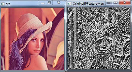
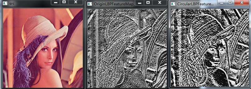
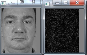
测试结果:
2、LBP特征的改进版本
在原始的LBP特征提出以后,研究人员对LBP特征进行了很多的改进,因此产生了许多LBP的改进版本。
2.1 圆形LBP特征(Circular LBP or Extended LBP)
由于原始LBP特征使用的是固定邻域内的灰度值,因此当图像的尺度发生变化时,LBP特征的编码将会发生错误,LBP特征将不能正确的反映像素点周围的纹理信息,因此研究人员对其进行了改进[3]。基本的 LBP 算子的最大缺陷在于它只覆盖了一个固定半径范围内的小区域,这显然不能满足不同尺寸和频率纹理的需要。为了适应不同尺度的纹理特征,并达到灰度和旋转不变性的要求,Ojala 等对 LBP 算子进行了改进,将 3×3 邻域扩展到任意邻域,并用圆形邻域代替了正方形邻域,改进后的 LBP 算子允许在半径为 R 的圆形邻域内有任意多个像素点。从而得到了诸如半径为R的圆形区域内含有P个采样点的LBP算子:
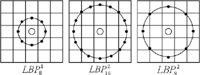
这种LBP特征叫做Extended LBP,也叫Circular LBP。使用可变半径的圆对近邻像素进行编码,可以得到如下的近邻:
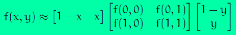
对于给定中心点(xc,yc)(xc,yc)用如下公式计算:
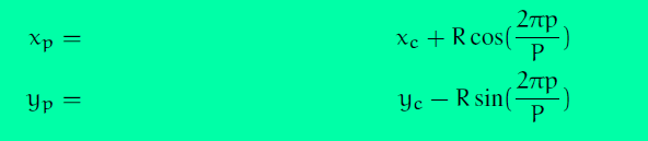
R是采样半径,p是第p个采样点,P是采样数目。由于计算的值可能不是整数,即计算出来的点不在图像上,我们使用计算出来的点的插值点。目的的插值方法有很多,Opencv使用的是双线性插值,双线性插值的公式如下:
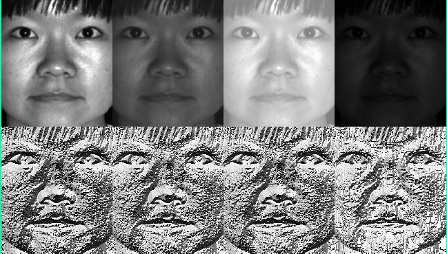
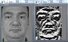
通过LBP特征的定义可以看出,LBP特征对光照变化是鲁棒的,其效果如下图所示:
//圆形LBP特征计算,这种方法适于理解,但在效率上存在问题,声明时默认neighbors=8
template <typename _tp>
void getCircularLBPFeature(InputArray _src,OutputArray _dst,int radius,int neighbors)
{
    Mat src = _src.getMat();
    //LBP特征图像的行数和列数的计算要准确
    _dst.create(src.rows-2*radius,src.cols-2*radius,CV_8UC1);
    Mat dst = _dst.getMat();
    dst.setTo(0);
    //循环处理每个像素
    for(int i=radius;i<src.rows-radius;i++)
    {
        for(int j=radius;j<src.cols-radius;j++)
        {
            //获得中心像素点的灰度值
            _tp center = src.at<_tp>(i,j);
            unsigned char lbpCode = 0;
            for(int k=0;k<neighbors;k++)
            {
                //根据公式计算第k个采样点的坐标,这个地方可以优化,不必每次都进行计算radius*cos,radius*sin
                float x = i + static_cast<float>(radius * \
                    cos(2.0 * CV_PI * k / neighbors));
                float y = j - static_cast<float>(radius * \
                    sin(2.0 * CV_PI * k / neighbors));
                //根据取整结果进行双线性插值,得到第k个采样点的灰度值

                //1.分别对x,y进行上下取整
                int x1 = static_cast<int>(floor(x));
                int x2 = static_cast<int>(ceil(x));
                int y1 = static_cast<int>(floor(y));
                int y2 = static_cast<int>(ceil(y));

                //2.计算四个点(x1,y1),(x1,y2),(x2,y1),(x2,y2)的权重
                //下面的权重计算方式有个问题,如果四个点都相等,则权重全为0,计算出来的插值为0
                //float w1 = (x2-x)*(y2-y); //(x1,y1)
                //float w2 = (x2-x)*(y-y1); //(x1,y2)
                //float w3 = (x-x1)*(y2-y); //(x2,y1)
                //float w4 = (x-x1)*(y-y1); //(x2,y2)

                //将坐标映射到0-1之间
                float tx = x - x1;
                float ty = y - y1;
                //根据0-1之间的x,y的权重计算公式计算权重
                float w1 = (1-tx) * (1-ty);
                float w2 =    tx  * (1-ty);
                float w3 = (1-tx) *    ty;
                float w4 =    tx  *    ty;
                //3.根据双线性插值公式计算第k个采样点的灰度值
                float neighbor = src.at<_tp>(x1,y1) * w1 + src.at<_tp>(x1,y2) *w2 \
                    + src.at<_tp>(x2,y1) * w3 +src.at<_tp>(x2,y2) *w4;
                //通过比较获得LBP值,并按顺序排列起来
                lbpCode |= (neighbor>center) <<(neighbors-k-1);
            }
            dst.at<uchar>(i-radius,j-radius) = lbpCode;
        }
    }
}
- 1
- 2
- 3
- 4
- 5
- 6
- 7
- 8
- 9
- 10
- 11
- 12
- 13
- 14
- 15
- 16
- 17
- 18
- 19
- 20
- 21
- 22
- 23
- 24
- 25
- 26
- 27
- 28
- 29
- 30
- 31
- 32
- 33
- 34
- 35
- 36
- 37
- 38
- 39
- 40
- 41
- 42
- 43
- 44
- 45
- 46
- 47
- 48
- 49
- 50
- 51
- 52
- 53
- 54
- 55
- 56
- 57
//圆形LBP特征计算,效率优化版本,声明时默认neighbors=8
template <typename _tp>
void getCircularLBPFeatureOptimization(InputArray _src,OutputArray _dst,int radius,int neighbors)
{
    Mat src = _src.getMat();
    //LBP特征图像的行数和列数的计算要准确
    _dst.create(src.rows-2*radius,src.cols-2*radius,CV_8UC1);
    Mat dst = _dst.getMat();
    dst.setTo(0);
    for(int k=0;k<neighbors;k++)
    {
        //计算采样点对于中心点坐标的偏移量rx,ry
        float rx = static_cast<float>(radius * cos(2.0 * CV_PI * k / neighbors));
        float ry = -static_cast<float>(radius * sin(2.0 * CV_PI * k / neighbors));
        //为双线性插值做准备
        //对采样点偏移量分别进行上下取整
        int x1 = static_cast<int>(floor(rx));
        int x2 = static_cast<int>(ceil(rx));
        int y1 = static_cast<int>(floor(ry));
        int y2 = static_cast<int>(ceil(ry));
        //将坐标偏移量映射到0-1之间
        float tx = rx - x1;
        float ty = ry - y1;
        //根据0-1之间的x,y的权重计算公式计算权重,权重与坐标具体位置无关,与坐标间的差值有关
        float w1 = (1-tx) * (1-ty);
        float w2 =    tx  * (1-ty);
        float w3 = (1-tx) *    ty;
        float w4 =    tx  *    ty;
        //循环处理每个像素
        for(int i=radius;i<src.rows-radius;i++)
        {
            for(int j=radius;j<src.cols-radius;j++)
            {
                //获得中心像素点的灰度值
                _tp center = src.at<_tp>(i,j);
                //根据双线性插值公式计算第k个采样点的灰度值
                float neighbor = src.at<_tp>(i+x1,j+y1) * w1 + src.at<_tp>(i+x1,j+y2) *w2 \
                    + src.at<_tp>(i+x2,j+y1) * w3 +src.at<_tp>(i+x2,j+y2) *w4;
                //LBP特征图像的每个邻居的LBP值累加,累加通过与操作完成,对应的LBP值通过移位取得
                dst.at<uchar>(i-radius,j-radius) |= (neighbor>center) <<(neighbors-k-1);
            }
        }
    }
}
- 1
- 2
- 3
- 4
- 5
- 6
- 7
- 8
- 9
- 10
- 11
- 12
- 13
- 14
- 15
- 16
- 17
- 18
- 19
- 20
- 21
- 22
- 23
- 24
- 25
- 26
- 27
- 28
- 29
- 30
- 31
- 32
- 33
- 34
- 35
- 36
- 37
- 38
- 39
- 40
- 41
- 42
- 43
- 44
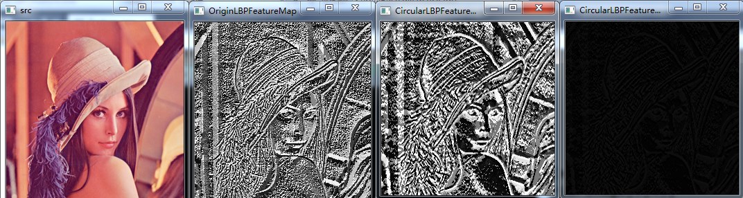
测试结果:
radius = 3,neighbors = 8
第三幅图像为radius = 3,neighbors = 8,第四幅图像为radius = 1,neighbors = 8,从实验结果可以看出,半径越小,图像纹理越精细
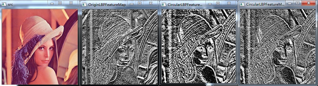
第三幅图像为radius = 3,neighbors = 8,第四幅图像为radius = 3,neighbors = 4,从实验结果可以看出,邻域数目越小,图像亮度越低,合理,因此4位的灰度值很小
由于我代码的问题,不能使neighbors >8,可改进
2.2 旋转不变LBP特征
从上面可以看出,上面的LBP特征具有灰度不变性,但还不具备旋转不变性,因此研究人员又在上面的基础上进行了扩展,提出了具有旋转不变性的LBP特征。
首先不断的旋转圆形邻域内的LBP特征,根据选择得到一系列的LBP特征值,从这些LBP特征值选择LBP特征值最小的作为中心像素点的LBP特征。具体做法如下图所示:
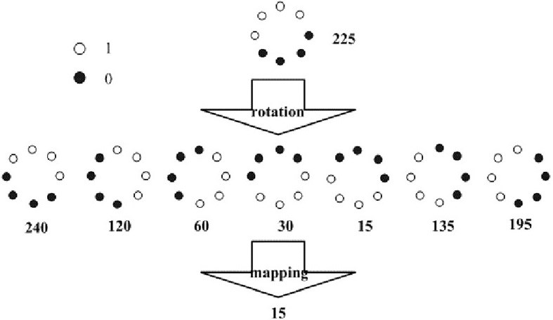
如图,通过对得到的LBP特征进行旋转,得到一系列的LBP特征值,最终将特征值最小的一个特征模式作为中心像素点的LBP特征。
//旋转不变圆形LBP特征计算,声明时默认neighbors=8
template <typename _tp>
void getRotationInvariantLBPFeature(InputArray _src,OutputArray _dst,int radius,int neighbors)
{
    Mat src = _src.getMat();
    //LBP特征图像的行数和列数的计算要准确
    _dst.create(src.rows-2*radius,src.cols-2*radius,CV_8UC1);
    Mat dst = _dst.getMat();
    dst.setTo(0);
    for(int k=0;k<neighbors;k++)
    {
        //计算采样点对于中心点坐标的偏移量rx,ry
        float rx = static_cast<float>(radius * cos(2.0 * CV_PI * k / neighbors));
        float ry = -static_cast<float>(radius * sin(2.0 * CV_PI * k / neighbors));
        //为双线性插值做准备
        //对采样点偏移量分别进行上下取整
        int x1 = static_cast<int>(floor(rx));
        int x2 = static_cast<int>(ceil(rx));
        int y1 = static_cast<int>(floor(ry));
        int y2 = static_cast<int>(ceil(ry));
        //将坐标偏移量映射到0-1之间
        float tx = rx - x1;
        float ty = ry - y1;
        //根据0-1之间的x,y的权重计算公式计算权重,权重与坐标具体位置无关,与坐标间的差值有关
        float w1 = (1-tx) * (1-ty);
        float w2 =    tx  * (1-ty);
        float w3 = (1-tx) *    ty;
        float w4 =    tx  *    ty;
        //循环处理每个像素
        for(int i=radius;i<src.rows-radius;i++)
        {
            for(int j=radius;j<src.cols-radius;j++)
            {
                //获得中心像素点的灰度值
                _tp center = src.at<_tp>(i,j);
                //根据双线性插值公式计算第k个采样点的灰度值
                float neighbor = src.at<_tp>(i+x1,j+y1) * w1 + src.at<_tp>(i+x1,j+y2) *w2 \
                    + src.at<_tp>(i+x2,j+y1) * w3 +src.at<_tp>(i+x2,j+y2) *w4;
                //LBP特征图像的每个邻居的LBP值累加,累加通过与操作完成,对应的LBP值通过移位取得
                dst.at<uchar>(i-radius,j-radius) |= (neighbor>center) <<(neighbors-k-1);
            }
        }
    }
    //进行旋转不变处理
    for(int i=0;i<dst.rows;i++)
    {
        for(int j=0;j<dst.cols;j++)
        {
            unsigned char currentValue = dst.at<uchar>(i,j);
            unsigned char minValue = currentValue;
            for(int k=1;k<neighbors;k++)
            {
    //循环左移
                unsigned char temp = (currentValue>>(neighbors-k)) | (currentValue<<k);
                if(temp < minValue)
                {
                    minValue = temp;
                }
            }
            dst.at<uchar>(i,j) = minValue;
        }
    }
}
- 1
- 2
- 3
- 4
- 5
- 6
- 7
- 8
- 9
- 10
- 11
- 12
- 13
- 14
- 15
- 16
- 17
- 18
- 19
- 20
- 21
- 22
- 23
- 24
- 25
- 26
- 27
- 28
- 29
- 30
- 31
- 32
- 33
- 34
- 35
- 36
- 37
- 38
- 39
- 40
- 41
- 42
- 43
- 44
- 45
- 46
- 47
- 48
- 49
- 50
- 51
- 52
- 53
- 54
- 55
- 56
- 57
- 58
- 59
- 60
- 61
- 62
- 63
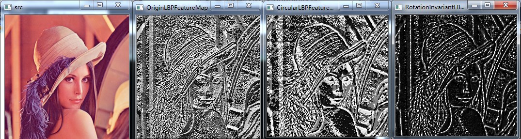
测试结果:
radius = 3,neighbors = 8,最后一幅是旋转不变LBP特征
2.3 Uniform Pattern LBP特征
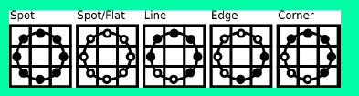
Uniform Pattern,也被称为等价模式或均匀模式,由于一个LBP特征有多种不同的二进制形式,对于半径为R的圆形区域内含有P个采样点的LBP算子将会产生2P2P种,共256个值,正好对应灰度图像的0-255,因此原始的LBP特征图像是一幅正常的灰度图像,而等价模式LBP特征,根据0-1跳变次数,将这256个LBP特征值分为了59类,从跳变次数上划分:跳变0次—2个,跳变1次—0个,跳变2次—56个,跳变3次—0个,跳变4次—140个,跳变5次—0个,跳变6次—56个,跳变7次—0个,跳变8次—2个。共9种跳变情况,将这256个值进行分配,跳变小于2次的为等价模式类,共58个,他们对应的值按照从小到大分别编码为1—58,即它们在LBP特征图像中的灰度值为1—58,而除了等价模式类之外的混合模式类被编码为0,即它们在LBP特征中的灰度值为0,因此等价模式LBP特征图像整体偏暗。
//等价模式LBP特征计算
template <typename _tp>
void getUniformPatternLBPFeature(InputArray _src,OutputArray _dst,int radius,int neighbors)
{
    Mat src = _src.getMat();
    //LBP特征图像的行数和列数的计算要准确
    _dst.create(src.rows-2*radius,src.cols-2*radius,CV_8UC1);
    Mat dst = _dst.getMat();
    dst.setTo(0);
    //LBP特征值对应图像灰度编码表,直接默认采样点为8位
    uchar temp = 1;
    uchar table[256] = {0};
    for(int i=0;i<256;i++)
    {
        if(getHopTimes(i)<3)
        {
            table[i] = temp;
            temp++;
        }
    }
    //是否进行UniformPattern编码的标志
    bool flag = false;
    //计算LBP特征图
    for(int k=0;k<neighbors;k++)
    {
        if(k==neighbors-1)
        {
            flag = true;
        }
        //计算采样点对于中心点坐标的偏移量rx,ry
        float rx = static_cast<float>(radius * cos(2.0 * CV_PI * k / neighbors));
        float ry = -static_cast<float>(radius * sin(2.0 * CV_PI * k / neighbors));
        //为双线性插值做准备
        //对采样点偏移量分别进行上下取整
        int x1 = static_cast<int>(floor(rx));
        int x2 = static_cast<int>(ceil(rx));
        int y1 = static_cast<int>(floor(ry));
        int y2 = static_cast<int>(ceil(ry));
        //将坐标偏移量映射到0-1之间
        float tx = rx - x1;
        float ty = ry - y1;
        //根据0-1之间的x,y的权重计算公式计算权重,权重与坐标具体位置无关,与坐标间的差值有关
        float w1 = (1-tx) * (1-ty);
        float w2 =    tx  * (1-ty);
        float w3 = (1-tx) *    ty;
        float w4 =    tx  *    ty;
        //循环处理每个像素
        for(int i=radius;i<src.rows-radius;i++)
        {
            for(int j=radius;j<src.cols-radius;j++)
            {
                //获得中心像素点的灰度值
                _tp center = src.at<_tp>(i,j);
                //根据双线性插值公式计算第k个采样点的灰度值
                float neighbor = src.at<_tp>(i+x1,j+y1) * w1 + src.at<_tp>(i+x1,j+y2) *w2 \
                    + src.at<_tp>(i+x2,j+y1) * w3 +src.at<_tp>(i+x2,j+y2) *w4;
                //LBP特征图像的每个邻居的LBP值累加,累加通过与操作完成,对应的LBP值通过移位取得
                dst.at<uchar>(i-radius,j-radius) |= (neighbor>center) <<(neighbors-k-1);
                //进行LBP特征的UniformPattern编码
                if(flag)
                {
                    dst.at<uchar>(i-radius,j-radius) = table[dst.at<uchar>(i-radius,j-radius)];
                }
            }
        }
    }
}
//计算跳变次数
int getHopTimes(int n)
{
    int count = 0;
    bitset<8> binaryCode = n;
    for(int i=0;i<8;i++)
    {
        if(binaryCode[i] != binaryCode[(i+1)%8])
        {
            count++;
        }
    }
    return count;
}
- 1
- 2
- 3
- 4
- 5
- 6
- 7
- 8
- 9
- 10
- 11
- 12
- 13
- 14
- 15
- 16
- 17
- 18
- 19
- 20
- 21
- 22
- 23
- 24
- 25
- 26
- 27
- 28
- 29
- 30
- 31
- 32
- 33
- 34
- 35
- 36
- 37
- 38
- 39
- 40
- 41
- 42
- 43
- 44
- 45
- 46
- 47
- 48
- 49
- 50
- 51
- 52
- 53
- 54
- 55
- 56
- 57
- 58
- 59
- 60
- 61
- 62
- 63
- 64
- 65
- 66
- 67
- 68
- 69
- 70
- 71
- 72
- 73
- 74
- 75
- 76
- 77
- 78
- 79
- 80
- 81
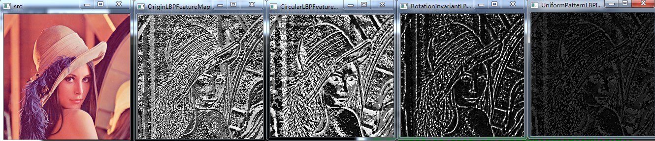
测试结果:
radius = 3,neighbors = 8,最后一幅是等价模式LBP特征
2.4 MB-LBP特征
MB-LBP特征,全称为Multiscale Block LBP,来源于论文[9],中科院的人发明的,在Traincascade级联目标训练检测中的LBP特征使用的就是MB-LBP。
MB-LBP的原理:
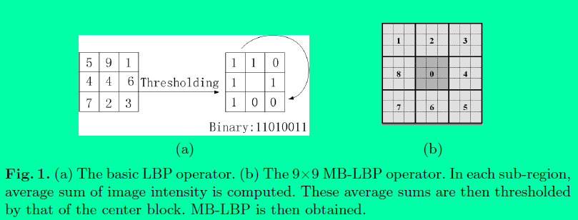
将图像分成一个个小块(Block),每个小块再分为一个个的小区域(类似于HOG中的cell),小区域内的灰度平均值作为当前小区域的灰度值,与周围小区域灰度进行比较形成LBP特征,生成的特征称为MB-LBP,Block大小为3*3,则小区域的大小为1,就是原始的LBP特征,上图的Block大小为9*9,小区域的大小为3*3。
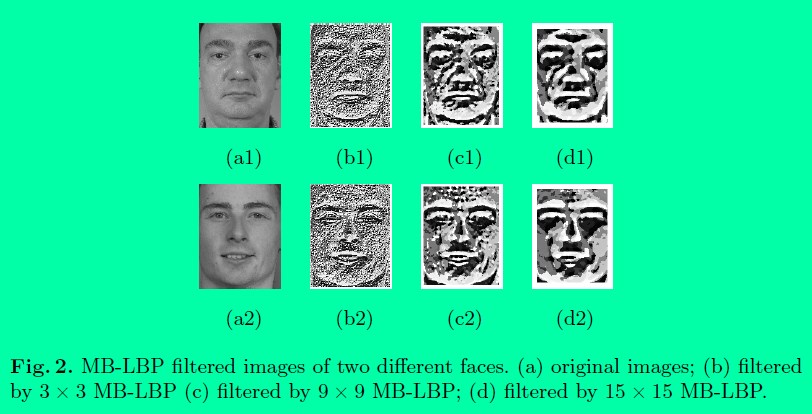
不同Block提取的MB-LBP特征如图所示:
计算MB-LBP代码:
//MB-LBP特征的计算
void getMultiScaleBlockLBPFeature(InputArray _src,OutputArray _dst,int scale)
{
    Mat src = _src.getMat();
    Mat dst = _dst.getMat();
    //定义并计算积分图像
    int cellSize = scale / 3;
    int offset = cellSize / 2;
    Mat cellImage(src.rows-2*offset,src.cols-2*offset,CV_8UC1);
    for(int i=offset;i<src.rows-offset;i++)
    {
        for(int j=offset;j<src.cols-offset;j++)
        {
            int temp = 0;
            for(int m=-offset;m<offset+1;m++)
            {
                for(int n=-offset;n<offset+1;n++)
                {
                    temp += src.at<uchar>(i+n,j+m);
                }
            }
            temp /= (cellSize*cellSize);
            cellImage.at<uchar>(i-cellSize/2,j-cellSize/2) = uchar(temp);
        }
    }
    getOriginLBPFeature<uchar>(cellImage,dst);
}
- 1
- 2
- 3
- 4
- 5
- 6
- 7
- 8
- 9
- 10
- 11
- 12
- 13
- 14
- 15
- 16
- 17
- 18
- 19
- 20
- 21
- 22
- 23
- 24
- 25
- 26
- 27
效果图:
Block=3,即原始的LBP特征
Block=9
Block=15
到此为止,还没有结束,作者对得到LBP特征又进行了均值模式编码,通过对得到的特征图求直方图,得到了LBP特征值0-255之间(0-255即直方图中的bin)的特征数量,通过对bin中的数值进行排序,通过权衡,将排序在前63位的特征值看作是等价模式类,其他的为混合模式类,总共64类,作者在论文中称之为SEMB-LBP(Statistically Effective MB-LBP )。类似于等价模式LBP,等价模式的LBP的等价模式类为58种,混合模式类1种,共59种。二者除了等价模式类的数量不同之外,主要区别在于:对等价模式类的定义不同,等价模式LBP是根据0-1的跳变次数定义的,而SEMB-LBP是通过对直方图排序得到的。当然下一步要做的就是将SEMB-LBP变为LBPH进行使用。
计算SEMB-LBP的代码
//求SEMB-LBP
void SEMB_LBPFeature(InputArray _src,OutputArray _dst,int scale)
{
    Mat dst=_dst.getMat();
    Mat MB_LBPImage;
    getMultiScaleBlockLBPFeature(_src,MB_LBPImage,scale);
    //imshow("dst",dst);
    Mat histMat;
    int histSize = 256;
    float range[] = {float(0),float(255)};
    const float* ranges = {range};
    //计算LBP特征值0-255的直方图
    calcHist(&MB_LBPImage,1,0,Mat(),histMat,1,&histSize,&ranges,true,false);
    histMat.reshape(1,1);
    vector<float> histVector(histMat.rows*histMat.cols);
    uchar table[256];
    memset(table,64,256);
    if(histMat.isContinuous())
    {
        //histVector = (int *)(histMat.data);
        //将直方图histMat变为vector向量histVector
        histVector.assign((float*)histMat.datastart,(float*)histMat.dataend);
        vector<float> histVectorCopy(histVector);
        //对histVector进行排序,即对LBP特征值的数量进行排序,降序排列
        sort(histVector.begin(),histVector.end(),greater<float>());
        for(int i=0;i<63;i++)
        {
            for(int j=0;j<histVectorCopy.size();j++)
            {
                if(histVectorCopy[j]==histVector[i])
                {
                    //得到类似于Uniform的编码表
                    table[j]=i;
                }
            }
        }
    }
    dst = MB_LBPImage;
    //根据编码表得到SEMB-LBP
    for(int i=0;i<dst.rows;i++)
    {
        for(int j=0;j<dst.cols;j++)
        {
            dst.at<uchar>(i,j) = table[dst.at<uchar>(i,j)];
        }
    }
}
- 1
- 2
- 3
- 4
- 5
- 6
- 7
- 8
- 9
- 10
- 11
- 12
- 13
- 14
- 15
- 16
- 17
- 18
- 19
- 20
- 21
- 22
- 23
- 24
- 25
- 26
- 27
- 28
- 29
- 30
- 31
- 32
- 33
- 34
- 35
- 36
- 37
- 38
- 39
- 40
- 41
- 42
- 43
- 44
- 45
- 46
- 47
测试结果:
第二幅为对MB-LBP进行编码得到的SEMB-LBP图像
总结:MB-LBP有点类似于先将图像进行平滑处理,然后再求LBP特征。而SEMB-LBP是在MB-LBP进行编码后的图像。类似于等价模式LBP,先求LBP特征,再用等价模式进行编码。当Scale=3时,MB-LBP和SEMB-LBP就是LBP和等价模式LBP。想具体了解需要去看论文,当然要自己实现才会理解的更透彻。
三、LBPH——图像的LBP特征向量
LBPH,Local Binary Patterns Histograms,即LBP特征的统计直方图,LBPH将LBP特征与图像的空间信息结合在一起。这种表示方法由Ahonen等人在论文[3]中提出,他们将LBP特征图像分成m个局部块,并提取每个局部块的直方图,然后将这些直方图依次连接在一起形成LBP特征的统计直方图,即LBPH。
一幅图像具体的计算LBPH的过程(以Opencv中的人脸识别为例):
1. 计算图像的LBP特征图像,在上面已经讲过了。
2. 将LBP特征图像进行分块,Opencv中默认将LBP特征图像分成8行8列64块区域
3. 计算每块区域特征图像的直方图cell_LBPH,将直方图进行归一化,直方图大小为1*numPatterns
4. 将上面计算的每块区域特征图像的直方图按分块的空间顺序依次排列成一行,形成LBP特征向量,大小为1*(numPatterns*64)
5. 用机器学习的方法对LBP特征向量进行训练,用来检测和识别目标
举例说明LBPH的维度:
采样点为8个,如果用的是原始的LBP或Extended LBP特征,其LBP特征值的模式为256种,则一幅图像的LBP特征向量维度为:64*256=16384维,
而如果使用的UniformPatternLBP特征,其LBP值的模式为59种,其特征向量维度为:64*59=3776维,可以看出,使用等价模式特征,其特征向量的维度大大减少,
这意味着使用机器学习方法进行学习的时间将大大减少,而性能上没有受到很大影响。
Opencv的人脸识别使用的是Extended LBP
计算LBPH的代码如下:
//计算LBP特征图像的直方图LBPH
Mat getLBPH(InputArray _src,int numPatterns,int grid_x,int grid_y,bool normed)
{
    Mat src = _src.getMat();
    int width = src.cols / grid_x;
    int height = src.rows / grid_y;
    //定义LBPH的行和列,grid_x*grid_y表示将图像分割成这么些块,numPatterns表示LBP值的模式种类
    Mat result = Mat::zeros(grid_x * grid_y,numPatterns,CV_32FC1);
    if(src.empty())
    {
        return result.reshape(1,1);
    }
    int resultRowIndex = 0;
    //对图像进行分割,分割成grid_x*grid_y块,grid_x,grid_y默认为8
    for(int i=0;i<grid_x;i++)
    {
        for(int j=0;j<grid_y;j++)
        {
            //图像分块
            Mat src_cell = Mat(src,Range(i*height,(i+1)*height),Range(j*width,(j+1)*width));
            //计算直方图
            Mat hist_cell = getLocalRegionLBPH(src_cell,0,(numPattern-1),true);
            //将直方图放到result中
            Mat rowResult = result.row(resultRowIndex);
            hist_cell.reshape(1,1).convertTo(rowResult,CV_32FC1);
            resultRowIndex++;
        }
    }
    return result.reshape(1,1);
}
//计算一个LBP特征图像块的直方图
Mat getLocalRegionLBPH(const Mat& src,int minValue,int maxValue,bool normed)
{
    //定义存储直方图的矩阵
    Mat result;
    //计算得到直方图bin的数目,直方图数组的大小
    int histSize = maxValue - minValue + 1;
    //定义直方图每一维的bin的变化范围
    float range[] = { static_cast<float>(minValue),static_cast<float>(maxValue + 1) };
    //定义直方图所有bin的变化范围
    const float* ranges = { range };
    //计算直方图,src是要计算直方图的图像,1是要计算直方图的图像数目,0是计算直方图所用的图像的通道序号,从0索引
    //Mat()是要用的掩模,result为输出的直方图,1为输出的直方图的维度,histSize直方图在每一维的变化范围
    //ranges,所有直方图的变化范围(起点和终点)
    calcHist(&src,1,0,Mat(),result,1,&histSize,&ranges,true,false);
    //归一化
    if(normed)
    {
        result /= (int)src.total();
    }
    //结果表示成只有1行的矩阵
    return result.reshape(1,1);
}
- 1
- 2
- 3
- 4
- 5
- 6
- 7
- 8
- 9
- 10
- 11
- 12
- 13
- 14
- 15
- 16
- 17
- 18
- 19
- 20
- 21
- 22
- 23
- 24
- 25
- 26
- 27
- 28
- 29
- 30
- 31
- 32
- 33
- 34
- 35
- 36
- 37
- 38
- 39
- 40
- 41
- 42
- 43
- 44
- 45
- 46
- 47
- 48
- 49
- 50
- 51
- 52
- 53
总结:上面的LBP特征都是较经典的LBP特征,除此之外,LBP特征还有大量的变种,如TLBP(中心像素与周围所有像素比较,而不是根据采样点的数目),DLBP(编码标准四个方向的灰度变化,每个方向上用2比特编码),MLBP(将中心像素值替换成采样点像素的平均值),MB-LBP(上面有介绍),VLBP(没太看懂),RGB-LBP(RGB图像分别计算LBP,然后连接在一起)等,具体的需要自己去研究,可参考维基百科
四、LBP特征的匹配与使用
1、LBP特征用在目标检测中
人脸检测比较出名的是Haar+Adaboost方法,其实目前的Opencv也支持LBP+Adaboost和HOG+Adaboost方法进行目标检测,从目前我的使用效果来看,LBP+Adaboost方法用在目标检测中的效果比Haar特征、HOG特征都要好(HOG特征用的不多,主要是Haar和LBP),而且LBP特征的训练速度比Haar和HOG都要快很多。在LBP+Adaboost中,LBP特征主要是用作输入的训练数据(特征),使用的LBP特征应该是DLBP(维基百科上说的,待考证,没太看明白Cascade中LBP特征的计算方式),具体用法需要看源码。Opencv的TrainCascade中使用的LBP特征是MB-LBP。
老外的对Opencv级联检测中使用的LBP的解释(非常好,自己读,就不翻译了),在看这个之前最好是运行过TrainCascade来训练目标检测的分类器,并使用过LBP特征训练,调节过参数[8]:
OpenCV ships with a tool called traincascade that trains LBP, Haar and HOG. Specifically for face detection they even ship the 3000-image dataset of 24x24 pixel faces, in the format needed bytraincascade.

In my experience, of the three types traincascade supports, LBP takes the least time to train, taking on the order of hours rather than days for Haar.

A quick overview of its training process is that for the given number of stages (a decent choice is 20), it attempts to find features that reject as many non-faces as possible while not rejecting the faces. The balance between rejecting non-faces and keeping faces is controlled by the mininum hit rate (OpenCV chose 99.5%) and false alarm rate (OpenCV chose 50%). The specific meta-algorithm used for crafting OpenCV's own LBP cascade is Gentle AdaBoost (GAB).

The variant of LBP implemented in OpenCV is described here:

Shengcai Liao, Xiangxin Zhu, Zhen Lei, Lun Zhang and Stan Z. Li. Learning Multi-scale Block Local Binary Patterns for Face Recognition. International Conference on Biometrics (ICB), 2007, pp. 828-837.

What it amounts to in practice in OpenCV with default parameters is:

OpenCV LBP Cascade Runtime Overview

The detector examines 24x24 windows within the image looking for a face. Stepping from Stage 1 to 20 of the cascade classifier, if it can show that the current 24x24 window is likely not a face, it rejects it and moves over the window by one or two pixels over to the next position; Otherwise it proceeds to the next stage.

During each stage, 3-10 or so LBP features are examined. Every LBP feature has an offset within the window and a size, and the area it covers is fully contained within the current window. Evaluating an LBP feature at a given position can result in either a pass or fail. Depending on whether an LBP feature succeeds or fails, a positive or negative weight particular to that feature is added to an accumulator.

Once all of a stage's LBP features are evaluated, the accumulator's value is compared to the stage threshold. A stage fails if the accumulator is below the threshold, and passes if it is above. Again, if a stage fails, the cascade is exited and the window moves to the next position.

LBP feature evaluation is relatively simple. At that feature's offset within the window, nine rectangles are laid out in a 3x3 configuration. These nine rectangles are all the same size for a particular LBP feature, ranging from 1x1 to 8x8.

The sum of all the pixels in the nine rectangles are computed, in other words their integral. Then, the central rectangle's integral is compared to that of its eight neighbours. The result of these eight comparisons is eight bits (1 or 0), which are assembled in an 8-bit LBP.

This 8-bit bitvector is used as an index into a 2^8 == 256-bit LUT, computed by the training process and particular to each LBP feature, that determines whether the LBP feature passed or failed.
- 1
- 2
- 3
- 4
- 5
- 6
- 7
- 8
- 9
- 10
- 11
- 12
- 13
- 14
- 15
- 16
- 17
- 18
- 19
- 20
- 21
- 22
- 23
- 24
- 25
- 26
2、 LBP用在人脸识别中
LBP在人脸识别中比较出名,从源码上来看,人脸识别中LBPH的使用主要是用来进行直方图的比较,通过直方图的比较来判断目标的类别。在Opencv的基于LBP的人脸识别的实现中使用的LBP特征是Extendes LBP,即圆形LBP特征。参考的论文为文献[10]。
LBPH训练主要是提取输入的图像的LBPH保存,当进行识别时,遍历保存的LBPH,找到输入图像与训练图像方差最小的LBPH,将其对应的类别作为识别的类别输出。
用LBPH进行训练和识别的代码。
#include<iostream>
#include<opencv2\core\core.hpp>
#include<opencv2\highgui\highgui.hpp>
#include<opencv2\imgproc\imgproc.hpp>
#include<opencv2\contrib\contrib.hpp>

using namespace std;
using namespace cv;

int main(int argc,char* argv[])
{
    vector<Mat> images;
    vector<int> labels;
    char buff[10];
    for(int i=1;i<8;i++)
    {
        sprintf(buff,"0%d.tif",i);
        Mat image = imread(buff);
        Mat grayImage;
        cvtColor(image,grayImage,COLOR_BGR2GRAY);
        images.push_back(grayImage);
        labels.push_back(1);
    }
    for(int i=8;i<12;i++)
    {
        sprintf(buff,"0%d.tif",i);
        Mat image = imread(buff);
        Mat grayImage;
        cvtColor(image,grayImage,COLOR_BGR2GRAY);
        images.push_back(grayImage);
        labels.push_back(2);
    }
    Ptr<FaceRecognizer> p = createLBPHFaceRecognizer();
    p->train(images,labels);
    Mat test= imread("12.tif");
    Mat grayImage;
    cvtColor(test,grayImage,COLOR_BGR2GRAY);
    int result = p->predict(grayImage);
    cout<<result<<endl;
    system("pause");
    return 0;
}
- 1
- 2
- 3
- 4
- 5
- 6
- 7
- 8
- 9
- 10
- 11
- 12
- 13
- 14
- 15
- 16
- 17
- 18
- 19
- 20
- 21
- 22
- 23
- 24
- 25
- 26
- 27
- 28
- 29
- 30
- 31
- 32
- 33
- 34
- 35
- 36
- 37
- 38
- 39
- 40
- 41
- 42
测试结果:

参考资料
[1] T. Ojala, M. Pietikäinen, and D. Harwood (1994), “Performance evaluation of texture measures with classification based on Kullback discrimination of distributions”, Proceedings of the 12th IAPR International Conference on Pattern Recognition (ICPR 1994), vol. 1, pp. 582 - 585.
[2] T. Ojala, M. Pietikäinen, and D. Harwood (1996), “A Comparative Study of Texture Measures with Classification Based on Feature Distributions”, Pattern Recognition, vol. 29, pp. 51-59.
[3] Ahonen, T., Hadid, A., and Pietikainen, M. Face Recognition with Local Binary Patterns. Computer Vision- ECCV 2004 (2004), 469–481.
[4] http://blog.csdn.net/xidianzhimeng/article/details/19634573
[5] opencv参考手册,Opencv源码
[6] http://blog.csdn.net/zouxy09/article/details/7929531
[7] http://blog.csdn.net/songzitea/article/details/17686135
[8] http://stackoverflow.com/questions/20085833/face-detection-algorithms-with-minimal-training-time/20086402#20086402
[9] Shengcai Liao, Xiangxin Zhu, Zhen Lei, Lun Zhang and Stan Z. Li. Learning Multi-scale Block Local Binary Patterns for Face Recognition. International Conference on Biometrics (ICB), 2007, pp. 828-837.
[10] Ahonen T, Hadid A. and Pietikäinen M. “Face description with local binary patterns: Application to face recognition.” IEEE Transactions on Pattern Analysis and Machine Intelligence, 28(12):2037-2041.


 3710
3710


 被折叠的 条评论
为什么被折叠?
被折叠的 条评论
为什么被折叠?
 到【灌水乐园】发言


