[R语言] 对diamonds数据集进行探索性数据分析（EDA）（——《来自数据科学》）

本文是对R的tidyverse包自带数据集diamonds进行探索。

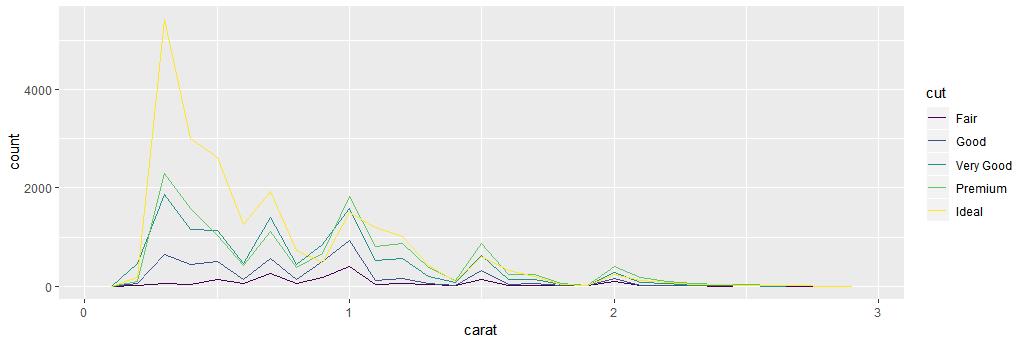
    #数据科学第5章——探索性数据分析 EDA
    library(tidyverse)
    smaller <- diamonds %>% filter(carat<3)#抽取克拉<3的数据
    ggplot(data = smaller,mapping = aes(x=carat,color = cut)) +
      geom_freqpoly(binwidth = 0.1)#频率多边形图探索克拉、切割的数据量

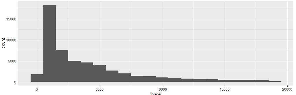
    max(diamonds$y)
    a <- select(diamonds,x,y,z)#选取x,y,z，探索常规统计量
    summary(a)
    ggplot(data = a,mapping = aes(x)) +
      geom_bar()
    ggplot(data = smaller,mapping = aes(x=price))+
      geom_histogram(binwidth = 1000)#直方图探索价格分布

count(diamonds[diamonds$carat==1,]) 1558

count(diamonds[diamonds$carat==0.99,]) 23 #比较克拉=1的钻石数量远高于0.99及其他非整数

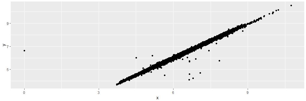
    ggplot(diamonds) +
      geom_histogram(mapping = aes(x=price)) +
      coord_cartesian(xlim = c(0,5000),ylim = c(0,7000))#定位x,y画布坐标范围
    #探索离群值点
    filter(diamonds,between(y,3,20))
    diamonds2 <- diamonds %>%
      mutate(y = ifelse(y<3 | y>20,NA,y))
    ggplot(data = diamonds2, mapping = aes(x = x, y = y)) +
      geom_point(na.rm=T)#散点图呈直线关系

    ggplot(data = diamonds2, mapping = aes(x = x, y = y)) +
      geom_smooth()
    ggplot(data = diamonds2, mapping = aes(x = y)) +
      geom_bar()#探索y的条形图
    ggplot(data = smaller) +
      geom_boxplot(mapping = aes(x = carat, y = price, group = cut_number(carat, 20)))#近似的显示每个分箱中的数据点的数量

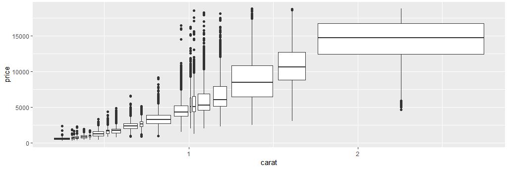价格随克拉数上升而上升，有较多的离群点

探索结论

克拉、切割、颜色、纯度对价格的影响是呈现线性正相关关系，同等条件下，克拉越高价格越高。