基于TensorFlow的Cats vs. Dogs（猫狗大战）实现和详解（2）

---

2018.9.4
更新完整Github代码：https://github.com/maples1993/Cats_vs_Dogs

---

2. 卷积神经网络模型的构造——model.py
　　关于神经网络模型不想说太多，视频中使用的模型是仿照TensorFlow的官方例程cifar-10的网络结构来写的。就是两个卷积层（每个卷积层后加一个池化层），两个全连接层，最后一个softmax输出分类结果。

import tensorflow as tf

def inference(images, batch_size, n_classes):
    # conv1, shape = [kernel_size, kernel_size, channels, kernel_numbers]
    with tf.variable_scope("conv1") as scope:
        weights = tf.get_variable("weights",
                                  shape=[3, 3, 3, 16],
                                  dtype=tf.float32,
                                  initializer=tf.truncated_normal_initializer(stddev=0.1, dtype=tf.float32))
        biases = tf.get_variable("biases",
                                 shape=[16],
                                 dtype=tf.float32,
                                 initializer=tf.constant_initializer(0.1))
        conv = tf.nn.conv2d(images, weights, strides=[1, 1, 1, 1], padding="SAME")
        pre_activation = tf.nn.bias_add(conv, biases)
        conv1 = tf.nn.relu(pre_activation, name="conv1")

    # pool1 && norm1
    with tf.variable_scope("pooling1_lrn") as scope:
        pool1 = tf.nn.max_pool(conv1, ksize=[1, 3, 3, 1], strides=[1, 2, 2, 1],
                               padding="SAME", name="pooling1")
        norm1 = tf.nn.lrn(pool1, depth_radius=4, bias=1.0, alpha=0.001/9.0,
                          beta=0.75, name='norm1')

    # conv2
    with tf.variable_scope("conv2") as scope:
        weights = tf.get_variable("weights",
                                  shape=[3, 3, 16, 16],
                                  dtype=tf.float32,
                                  initializer=tf.truncated_normal_initializer(stddev=0.1, dtype=tf.float32))
        biases = tf.get_variable("biases",
                                 shape=[16],
                                 dtype=tf.float32,
                                 initializer=tf.constant_initializer(0.1))
        conv = tf.nn.conv2d(norm1, weights, strides=[1, 1, 1, 1], padding="SAME")
        pre_activation = tf.nn.bias_add(conv, biases)
        conv2 = tf.nn.relu(pre_activation, name="conv2")

    # pool2 && norm2
    with tf.variable_scope("pooling2_lrn") as scope:
        pool2 = tf.nn.max_pool(conv2, ksize=[1, 3, 3, 1], strides=[1, 2, 2, 1],
                               padding="SAME", name="pooling2")
        norm2 = tf.nn.lrn(pool2, depth_radius=4, bias=1.0, alpha=0.001/9.0,
                          beta=0.75, name='norm2')

    # full-connect1
    with tf.variable_scope("fc1") as scope:
        reshape = tf.reshape(norm2, shape=[batch_size, -1])
        dim = reshape.get_shape()[1].value
        weights = tf.get_variable("weights",
                                  shape=[dim, 128],
                                  dtype=tf.float32,
                                  initializer=tf.truncated_normal_initializer(stddev=0.005, dtype=tf.float32))
        biases = tf.get_variable("biases",
                                 shape=[128],
                                 dtype=tf.float32,
                                 initializer=tf.constant_initializer(0.1))
        fc1 = tf.nn.relu(tf.matmul(reshape, weights) + biases, name="fc1")

    # full_connect2
    with tf.variable_scope("fc2") as scope:
        weights = tf.get_variable("weights",
                                  shape=[128, 128],
                                  dtype=tf.float32,
                                  initializer=tf.truncated_normal_initializer(stddev=0.005, dtype=tf.float32))
        biases = tf.get_variable("biases",
                                 shape=[128],
                                 dtype=tf.float32,
                                 initializer=tf.constant_initializer(0.1))
        fc2 = tf.nn.relu(tf.matmul(fc1, weights) + biases, name="fc2")

    # softmax
    with tf.variable_scope("softmax_linear") as scope:
        weights = tf.get_variable("weights",
                                  shape=[128, n_classes],
                                  dtype=tf.float32,
                                  initializer=tf.truncated_normal_initializer(stddev=0.005, dtype=tf.float32))
        biases = tf.get_variable("biases",
                                 shape=[n_classes],
                                 dtype=tf.float32,
                                 initializer=tf.constant_initializer(0.1))
        softmax_linear = tf.add(tf.matmul(fc2, weights), biases, name="softmax_linear")
        softmax_linear = tf.nn.softmax(softmax_linear)
    return softmax_linear

　　发现程序里面有很多with tf.variable_scope("name")的语句，这其实是TensorFlow中的变量作用域机制，目的是有效便捷地管理需要的变量。
　　变量作用域机制在TensorFlow中主要由两部分组成：

• tf.get_variable(<name>, <shape>, <initializer>): 创建一个变量
• tf.variable_scope(<scope_name>): 指定命名空间

如果需要共享变量，需要通过reuse_variables()方法来指定，详细的例子去官方文档中看就好了。（链接在博客参考部分）

def losses(logits, labels):
    with tf.variable_scope("loss") as scope:
        cross_entropy = tf.nn.sparse_softmax_cross_entropy_with_logits(logits=logits,
                                                                       labels=labels, name="xentropy_per_example")
        loss = tf.reduce_mean(cross_entropy, name="loss")
        tf.summary.scalar(scope.name + "loss", loss)
    return loss


def trainning(loss, learning_rate):
    with tf.name_scope("optimizer"):
        optimizer = tf.train.AdamOptimizer(learning_rate=learning_rate)
        global_step = tf.Variable(0, name="global_step", trainable=False)
        train_op = optimizer.minimize(loss, global_step=global_step)
    return train_op


def evaluation(logits, labels):
    with tf.variable_scope("accuracy") as scope:
        correct = tf.nn.in_top_k(logits, labels, 1)
        correct = tf.cast(correct, tf.float16)
        accuracy = tf.reduce_mean(correct)
        tf.summary.scalar(scope.name + "accuracy", accuracy)
    return accuracy

　　 函数losses(logits, labels)用于计算训练过程中的loss，这里输入参数logtis是函数inference()的输出，代表图片对猫和狗的预测概率，labels则是图片对应的标签。
　　通过在程序中设置断点，查看logtis的值，结果如下图所示，根据这个就很好理解了，一个数值代表属于猫的概率，一个数值代表属于狗的概率，两者的和为1。

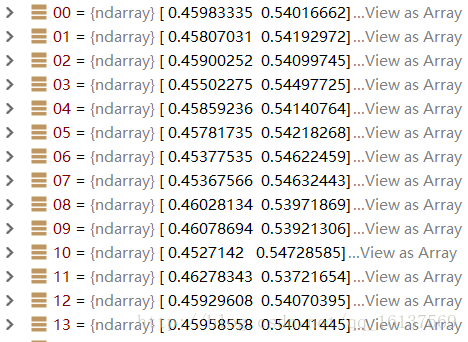
　　而函数tf.nn.sparse_sotfmax_cross_entropy_with_logtis从名字就很好理解，是将稀疏表示的label与输出层计算出来结果做对比。然后因为训练的时候是16张图片一个batch，所以再用tf.reduce_mean求一下平均值，就得到了这个batch的平均loss。
　　training(loss, learning_rate)就没什么好说的了，loss是训练的loss，learning_rate是学习率，使用AdamOptimizer优化器来使loss朝着变小的方向优化。
　　evaluation(logits, labels)功能是在训练过程中实时监测验证数据的准确率，达到反映训练效果的作用。

参考

---

1. TensorFlow官方文档 | 共享变量

补充

　　本来是自己之前犯懒，最后一篇关于训练的博客没写=0=，鉴于不少人想要训练代码，这里我就从简贴一下代码好了，大伙将就着看看，最近自己的事比较多，不想再把最开始的代码拿来翻了（刚开始写的太丑了）。

import os
import numpy as np
import tensorflow as tf
import input_data
import model

N_CLASSES = 2
IMG_H = 208
IMG_W = 208
BATCH_SIZE = 32
CAPACITY = 2000
MAX_STEP = 15000
learning_rate = 0.0001


def run_training():
    train_dir = "data\\train\\"
    logs_train_dir = "logs\\"

    train, train_label = input_data.get_files(train_dir)
    train_batch, train_label_batch = input_data.get_batch(train,
                                                          train_label,
                                                          IMG_W,
                                                          IMG_H,
                                                          BATCH_SIZE,
                                                          CAPACITY)
    train_logits = model.inference(train_batch, BATCH_SIZE, N_CLASSES)
    train_loss = model.losses(train_logits, train_label_batch)
    train_op = model.trainning(train_loss, learning_rate)
    train_acc = model.evaluation(train_logits, train_label_batch)

    summary_op = tf.summary.merge_all()
    sess = tf.Session()
    train_writer = tf.summary.FileWriter(logs_train_dir, sess.graph)
    saver = tf.train.Saver()

    sess.run(tf.global_variables_initializer())
    coord = tf.train.Coordinator()
    threads = tf.train.start_queue_runners(sess=sess, coord=coord)

    try:
        for step in np.arange(MAX_STEP):
            if coord.should_stop():
                break
            _, tra_loss, tra_acc = sess.run([train_op, train_loss, train_acc])

            if step % 100 == 0:
                print("Step %d, train loss = %.2f, train accuracy = %.2f%%" % (step, tra_loss, tra_acc))
                summary_str = sess.run(summary_op)
                train_writer.add_summary(summary_str, step)
            if step % 2000 == 0 or (step + 1) == MAX_STEP:
                checkpoint_path = os.path.join(logs_train_dir, "model.ckpt")
                saver.save(sess, checkpoint_path, global_step=step)
    except tf.errors.OutOfRangeError:
        print("Done training -- epoch limit reached.")
    finally:
        coord.request_stop()

    coord.join(threads)
    sess.close()

# 评估模型
from PIL import Image
import matplotlib.pyplot as plt


def get_one_image(train):
    n = len(train)
    ind = np.random.randint(0, n)
    img_dir = train[ind]

    image = Image.open(img_dir)
    plt.imshow(image)
    plt.show()
    image = image.resize([208, 208])
    image = np.array(image)
    return image


def evaluate_one_image():
    train_dir = "C:\\Users\\panch\\Documents\\PycharmProjects\\Cats_vs_Dogs\\data\\train\\"
    train, train_label = input_data.get_files(train_dir)
    image_array = get_one_image(train)

    with tf.Graph().as_default():
        BATCH_SIZE = 1
        N_CLASSES = 2

        image = tf.cast(image_array, tf.float32)
        image = tf.reshape(image, [1, 208, 208, 3])
        logit = model.inference(image, BATCH_SIZE, N_CLASSES)
        logit = tf.nn.softmax(logit)

        x = tf.placeholder(tf.float32, shape=[208, 208, 3])

        logs_train_dir = "C:\\Users\\panch\\Documents\\PycharmProjects\\Cats_vs_Dogs\\logs\\"
        saver = tf.train.Saver()

        with tf.Session() as sess:
            print("Reading checkpoints...")
            ckpt = tf.train.get_checkpoint_state(logs_train_dir)
            if ckpt and ckpt.model_checkpoint_path:
                global_step = ckpt.model_checkpoint_path.split("/")[-1].split("-")[-1]
                saver.restore(sess, ckpt.model_checkpoint_path)
                print("Loading success, global_step is %s" % global_step)
            else:
                print("No checkpoint file found")

            prediction = sess.run(logit, feed_dict={x: image_array})
            max_index = np.argmax(prediction)
            if max_index == 0:
                print("This is a cat with possibility %.6f" % prediction[:, 0])
            else:
                print("This is a dog with possibility %.6f" % prediction[:, 1])


run_training()
# evaluate_one_image()