pytorch学习笔记（二)(补充)

简单数据分类实验

这里记录一下莫烦视频的分类实验，一个平面上的离散数据的分类。

数据制造

torch.normal(*mean*, *std*, ***, *generator=None*, *out=None*) → Tensor

离散正态分布，其中mean和std都可以是多维数据。可以：

mean多维，std一维；mean一维，std多维；或者mean与std的维数相同

torch.normal(mean=torch.arange(0,11), std=0.5)
torch.normal(mean=0.5, std=torch.arange(1., 6.))
torch.normal(mean=torch.arange(0,11), std=torch.arange(0,1,0.1))

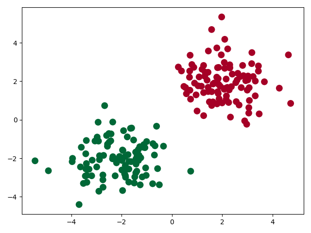
分别创建了200对（x，y）数据，根据二维正态分布在（-2，-2）和（2，2）处

# 假数据
n_data = torch.ones(100, 2)         # 数据的基本形态
x0 = torch.normal(2*n_data, 1)      # 类型0 x data (tensor), shape=(100, 2)
y0 = torch.zeros(100)               # 类型0 y data (tensor), shape=(100, )
x1 = torch.normal(-2*n_data, 1)     # 类型1 x data (tensor), shape=(100, 1)
y1 = torch.ones(100)                # 类型1 y data (tensor), shape=(100, )
# 注意 x, y 数据的数据形式是一定要像下面一样 (torch.cat 是在合并数据)
x = torch.cat((x0, x1), 0).type(torch.FloatTensor)  # FloatTensor = 32-bit floating
#规定标签一点要是LongTensor
y = torch.cat((y0, y1), ).type(torch.LongTensor)    # LongTensor = 64-bit integer

#这里就是绘制散点图，其中cmap是一种颜色映射图，我的csdn收藏里有
plt.scatter(x.data.numpy()[:, 0], x.data.numpy()[:, 1], c=y.data.numpy(), s=100, lw=0, cmap='RdYlGn')
plt.show()

网路搭建

这里的网络搭建跟上一次没什么区别。

class Net(nn.Module):
    def __init__(self,in_feature,out):
        super(Net,self).__init__()
        #construct net
        self.hidden1=nn.Linear(in_feature,100)
        self.hidden2=nn.Linear(100,20)
        self.predict=nn.Linear(20,out)

    def forward(self, x):
        x=F.relu(self.hidden1(x))
        x = F.relu(self.hidden2(x))
        x=self.predict(x)
        return x

优化器与损失函数

这里做一点关于损失函数的交叉解释：

• MSELoss（）多用于回归问题，也可以用于one_hotted编码形式，要求batch_x与batch_y的tensor都是FloatTensor类型；
• CrossEntropyLoss()，多用于分类问题，名字为交叉熵损失函数，不用于one_hotted编码形式，要求batch_x为Float，batch_y为LongTensor类型

net=Net(2,2)
print(net)
optimizer = torch.optim.SGD(net.parameters(), lr=0.02)  # 传入 net 的所有参数, 学习率
# 算误差的时候, 注意真实值!不是! one-hot 形式的, 而是1D Tensor, (batch,)
# 但是预测值是2D tensor (batch, n_classes)
loss_func = torch.nn.CrossEntropyLoss()

训练与输出

这里说明一下softmax函数：

torch.nn.functional.softmax(input, dim=None, _stacklevel=3, dtype=None)

作用就是：$\mathrm{Softmax}\left(x_i\right)=\frac{\exp \left(x_i\right)}{{\sum }_j\exp \left(x_j\right)}$

将某一轴上的数据，以概率值输入，概率相加等于1，其中dim参数:指定对哪一轴进行softmax，比如2*2的tensor，dim=0，就是对列求softmax，dim=1就是对行求softmax。

a=torch.randn(2,2)
print(a)
b=F.softmax(a,dim=0)
print(b)
>>>>>>>>>>
tensor([[-1.7032, -0.7154],
        [-0.9984,  0.4077]])
tensor([[0.3307, 0.2454],
        [0.6693, 0.7546]])

另外CrossEntropyLoss()为损失函数的输入为：out.size()=(batch,classes);y.size()=(batch)，因为以下公式

$\mathrm{loss}(x,\text{ class })=-\log \left(\frac{\exp (x[\text{ class }])}{{\sum }_j\exp (x[j])}\right)=-x[\text{ class }]+\log \left({\sum }_j\exp (x[j])\right)$，对于一个数据来说，会预测出classes个类别，但是标签值不应该用one-hot来表示，所以会少一维。

for t in range(100):
    out = net(x)     # 喂给 net 训练数据 x, 输出分析值
    loss = loss_func(out, y)     # 计算两者的误差
    optimizer.zero_grad()   # 清空上一步的残余更新参数值
    loss.backward()
    optimizer.step()
    if t % 2 == 0:
        plt.cla()
        # 过了一道 softmax 的激励函数后的最大概率才是预测值
        prediction = torch.max(F.softmax(out), 1)[1]
        pred_y = prediction.data.numpy().squeeze()
        target_y = y.data.numpy()
        plt.scatter(x.data.numpy()[:, 0], x.data.numpy()[:, 1], c=pred_y, s=100, lw=0, cmap='RdYlGn')
        accuracy = sum(pred_y == target_y)/200.  # 预测中有多少和真实值一样
        plt.text(1.5, -4, 'Accuracy=%.2f' % accuracy, fontdict={'size': 20, 'color':  'red'})
        plt.pause(0.1)

plt.ioff()  # 停止画图

结果：

完整代码：https://github.com/UESTC-Liuxin/pytorch/blob/master/Exp7.py