python之客户逾期还款业务

最新推荐文章于 2021-09-30 18:41:31 发布

数据分析痴迷者

最新推荐文章于 2021-09-30 18:41:31 发布

阅读量1.8k

点赞数 1

分类专栏：机器学习文章标签： python 机器学习数据分析

本文链接：https://blog.csdn.net/qq_21573621/article/details/105959808

版权

机器学习专栏收录该内容

3 篇文章 0 订阅

订阅专栏

数据源结构：数据集是Lending Club平台发生借贷的业务数据，共有52个变量，39522条记录。

1、数据预处理

去掉一些明显没用的特征。

import pandas as pd
import numpy as np
import matplotlib.pyplot as plt
import seaborn as sns
import warnings

warnings.filterwarnings('ignore') #忽视错误

loans = pd.read_csv('./LoanStats3a.csv', skiprows=1) #第一行是字符串，所以要skiprows=1跳过第一行
half_count = len(loans) / 2 # 4万行除以2 = 19767.5行

loans = loans.dropna(thresh=half_count, axis=1)#2万行中剔除空白值超过一半的列，thresh：剔除
loans = loans.drop(['desc', 'url'],axis=1) #按照列中，删除描述和URL链接
loans.to_csv('loans.csv', index=False) #追加到“loans.csv”文件 ， index=False#表示不加索引

loans = pd.read_csv("./loans.csv")#读取数据
#数据的特征名
loans.columns

从常识来讲‘id’和‘member_id’与银行是否对他进行放贷没有任何关系，’funded_amnt(期望贷款的值)’ 和funded_amnt_inv(实际发放的款数)’为预测之后银行对该人借贷的金额，很明显也与模型判断没有关系。

#id：用户ID
#member_id：会员编号
#funded_amnt：承诺给该贷款的总金额
#funded_amnt_inv：投资者为该贷款承诺的总金额
#grade：贷款等级。贷款利率越高，则等级越高
#sub_grade：贷款子等级
#emp_title：工作名称
#issue_d：贷款月份
loans = loans.drop(["id", "member_id", "funded_amnt", "funded_amnt_inv", "grade", "sub_grade", "emp_title", "issue_d"], axis=1)

#zip_code：常用的邮编
#out_prncp和out_prncp_inv都是一样的：总资金中剩余的未偿还本金
#out_prncp_inv：实际未偿还的本金
#total_rec_prncp：迄今收到的本金

loans = loans.drop(["zip_code", "out_prncp", "out_prncp_inv", "total_pymnt", "total_pymnt_inv", "total_rec_prncp"], axis=1)

#total_rec_int：迄今收到的利息

#recoveries：是否收回本金
#collection_recovery_fee：收集回收费用
#last_pymnt_d：最近一次收到还款的时间
#last_pymnt_amnt：全部的还款的时间

loans = loans.drop(["total_rec_int", "total_rec_late_fee", "recoveries", "collection_recovery_fee", "last_pymnt_d", "last_pymnt_amnt"], axis=1)

确定当前贷款状态

print(loans['loan_status'].value_counts())#计算该列特征的属性的个数


#Fully Paid：批准了客户的贷款，后面给他打个“1”
#Charged Off：没有批准了客户的贷款，后面给他打个“0”
#Does not meet the credit policy. Status:Fully Paid：，没有满足要求的有1988个，也不要说清楚不贷款，就不要这个属性了
#后面的属性不确定比较强
#Late (16-30 days)  ：延期了16-30 days
#Late (31-120 days)：延期了31-120 days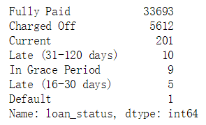

#要做一个二分类，用0 1 表示
loans = loans[(loans['loan_status'] == "Fully Paid") |
                        (loans['loan_status'] == "Charged Off")]
status_replace = {
    #特征当做key，value里还有一个字典
    "loan_status": {
        #第一个键值改为1 ，第二个键值改为0
        "Fully Paid": 1, #完全支付
        "Charged Off": 0,#违约
    }
}
#可以用pandas的DataFrame的格式，做成字典

loans = loans.replace(status_replace)  #replace：执行的是查找并替换的操作

去掉特征中只有一种属性的列

#在原始数据中的特征值或者属性里都是一样的，对于分类模型的预测是没有用的
#某列特征都是n n n  NaN  n n ,有缺失的，唯一的属性就有2个，用pandas空值给去掉

orig_columns = loans.columns  #展现出所有的列

drop_columns = []  #初始化空值

for col in orig_columns:
    #   dropna()先删除空值，再去重算唯一的属性
    col_series = loans[col].dropna().unique()  #去重唯一的属性
    if len(col_series) == 1:  #如果该特征的属性只有一个属性，就给过滤掉该特征
        drop_columns.append(col)
        
loans = loans.drop(drop_columns, axis=1)
print(drop_columns)
print("--------------------------------------------")
print(loans.shape)
loans.to_csv('./filtered_loans.csv', index=False)

#还剩下24个候选特征

处理缺失值

loans = pd.read_csv('./filtered_loans.csv')
null_counts = loans.isnull().sum()  #用pandas的isnull统计一下每列的缺失值，给累加起来

从统计出的结果可以看出‘title’和‘revol_util’相对于数据总量来说较少，可以直接去掉缺失值所在的行，而‘pub_rec_bankruptcies ’中的缺失值较多，说明该数据统计的情况较差，直接将此特征删除即可。

loans = loans.drop("pub_rec_bankruptcies", axis=1)
loans = loans.dropna(axis=0) 
#用dtypes类型统计有多少个是object、int、float类型的特征
print(loans.dtypes.value_counts())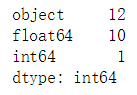

数据类型的转换

#Pandas里select_dtypes只选定“ohbject”的类型str，只选定字符型的数据

object_columns_df = loans.select_dtypes(include=["object"])
print(object_columns_df.iloc[0])


#term：分期多少个月啊
#int_rate：利息，10.65%，后面还要把%去掉
#emp_length：10年的映射成10，9年的映射成9
#home_ownership：房屋所有权，是租的、还是自己的、还是低压出去了，那就用0 1 2来代替

#labelencoder
# jemp_length做成字典，emp_length当做key ，value里还是字典 ，"10+ years": 10...
# 再在后面调用replace函数，刚才利息这列特征，是不是有%啊，再用astype()处理一下

mapping_dict = {
    "emp_length": {
        "10+ years": 10,
        "9 years": 9,
        "8 years": 8,
        "7 years": 7,
        "6 years": 6,
        "5 years": 5,
        "4 years": 4,
        "3 years": 3,
        "2 years": 2,
        "1 year": 1,
        "< 1 year": 0,
        "n/a": 0
    }
}

# 删除：last_credit_pull_d：LC撤回最近的月份   
#earliest_cr_line：第一次借贷时间
#addr_state：家庭邮编
#title：URL的标题
loans = loans.drop(
    ["last_credit_pull_d", "earliest_cr_line", "addr_state", "title"], axis=1)
#rstrip：删除 string 字符串末尾的指定字符
loans["int_rate"] = loans["int_rate"].str.rstrip("%").astype("float")
#revol_util：透支额度占信用比例
loans["revol_util"] = loans["revol_util"].str.rstrip("%").astype("float")
loans = loans.replace(mapping_dict)

剩余的其他字符型特征，此处选择使用pandas的get_dummies()函数，直接映射为数值型。

#查看指定标签的属性，并记数
#home_ownership：房屋所有权
#verification_status：身份保持证明
#emp_length：客户公司名称
#purpose：贷款的意图
#term：贷款分期的时间

cat_columns = ["home_ownership", "verification_status", "emp_length", "purpose", "term"]
dummy_df = pd.get_dummies(loans[cat_columns])
#concat() 方法用于连接两个或多个数组,
loans = pd.concat([loans, dummy_df], axis=1)
loans = loans.drop(cat_columns, axis=1)
#pymnt_plan 指示是否已为贷款实施付款计划 ，里面都为N，删掉这一列
loans = loans.drop("pymnt_plan", axis=1)

loans.to_csv('./cleaned_loans_2020.csv', index=False)

什么时候用OneHotEncoder独热编码和LabelEncoder标签编码？

特征的属性小于等于3 ，就用OneHotEncoder，比如说：天气、性别，属于无序特征
特征的属性大于3，就用LabelEncoder，比如说：星期，属于有序型

loans = pd.read_csv("cleaned_loans_2020.csv") # 清洗完的数据拿过来，现在的数据要么是float类型和int类型

模型训练

前面花费了大量的时间在进行数据处理，这足以说明在机器学习中数据准备的工作有多重要，有了好的数据才能预测出好的分类结果，对于二分类问题，一般情况下，首选逻辑回归。
首先定义模型效果的评判标准。根据贷款行业的实际情况，在这里我们假设将钱借给了没有还款能力的人，结果损失一千，将钱借给了有偿还能力的人，从每笔中赚0.1的利润，而其余情况收益为零，就相当于预测对十个人才顶上预测错一个人的收益，所以精度不再适用于此模型，为了实现利润最大化，不仅要求模型预测recall率较高，同时是需要要让fall-out率较低，故这里采用两个指标TPR(true positive rate)和FPR(false positive rate)。

from sklearn.linear_model import LogisticRegression # 分类
lr = LogisticRegression() # 调用逻辑回归的算法包


cols = loans.columns # 4万行 * 24列的样本
train_cols = cols.drop("loan_status") # 删除loan_status这一列作为目标值

features = loans[train_cols] # 23列的特征矩阵
target = loans["loan_status"] # 作为标签矩阵

lr.fit(features, target) #开始训练
predictions = lr.predict(features) # 开始预测

#接下来就是如何算4个指标 fp tp fn tn

# 假正类（False Positive，FP）：将负类预测为正类
fp_filter = (predictions == 1) & (loans["loan_status"] == 0)
fp = len(predictions[fp_filter])
print(fp)
print("----------------------------------------")


# 真正类（True Positive，TP）：将正类预测为正类
tp_filter = (predictions == 1) & (loans["loan_status"] == 1)
tp = len(predictions[tp_filter])
print(tp)
print("----------------------------------------")


# 假负类（False Negative，FN）：将正类预测为负类
fn_filter = (predictions == 0) & (loans["loan_status"] == 1)
fn = len(predictions[fn_filter])
print(fn)
print("----------------------------------------")

# 真负类（True Negative，TN）：将负类预测为负类
tn_filter = (predictions == 0) & (loans["loan_status"] == 0)
tn = len(predictions[tn_filter])
print(tn)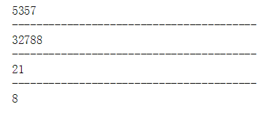

from sklearn.linear_model import LogisticRegression
from sklearn.model_selection import cross_val_predict

lr = LogisticRegression()
predictions = cross_val_predict(lr, features, target, cv=10) # Kfold = 10(交叉验证)
predictions = pd.Series(predictions)
print(predictions[:1000])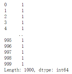

# 假正类（False Positive，FP）：将负类预测为正类
fp_filter = (predictions == 1) & (loans["loan_status"] == 0)
fp = len(predictions[fp_filter])


# 真正类（True Positive，TP）：将正类预测为正类
tp_filter = (predictions == 1) & (loans["loan_status"] == 1)
tp = len(predictions[tp_filter])



# 假负类（False Negative，FN）：将正类预测为负类
fn_filter = (predictions == 0) & (loans["loan_status"] == 1)
fn = len(predictions[fn_filter])



# 真负类（True Negative，TN）：将负类预测为负类
tn_filter = (predictions == 0) & (loans["loan_status"] == 0)
tn = len(predictions[tn_filter])

# Rates：就可以用刚才的指标进行衡量了呀
tpr = tp / float((tp + fn))
fpr = fp / float((fp + tn))
"""
tpr:比较高，我们非常喜欢，给他贷款了，而且这些人能还钱了
fpr：比较高，这些人不会还钱，但还是贷给他了吧
为什么这个2个值都那么高呢？把所有人来了，都借给他钱呀，打印出前20行都为1，为什么会出现这种情况？
绝对是前面的数据出现问题了，比如说数据是6：1，绝大多数是1，小部分是0，样本不均衡的情况下，导致分类器错误的认为把所有的样本预测为1，因为负样本少，咱们就“数据增强”，
把负样本1增强到4份儿，是不是可以啊，要么收集数据 ，数据已经定值了，没办法收集，要么是造数据，你知道什么样的人会还钱吗？也不好造吧，怎么解决样本不均衡的问题呢？
接下来要考虑权重的东西了，一部分是6份，另一部分是1份，把6份的权重设置为1，把1份的权重设置为6，设置权重项来进行衡量，把不均衡的样本变得均衡，加了权重项，让正样本对结果的影响小一些，
让负样本对结果的影响大一些，通过加入权重项，模型对结果变得均衡一下，有一个参数很重要
"""
print(tpr)#真正率
print(fpr)#假正率
print(predictions[:20])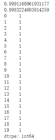

from sklearn.linear_model import LogisticRegression
from sklearn.model_selection import cross_val_predict
"""
class_weight：可以调整正反样本的权重
balanced:希望正负样本平衡一些的
"""
lr = LogisticRegression(class_weight="balanced")
predictions = cross_val_predict(lr, features, target, cv=10)
predictions = pd.Series(predictions)

# False positives.
fp_filter = (predictions == 1) & (loans["loan_status"] == 0)
fp = len(predictions[fp_filter])

# True positives.
tp_filter = (predictions == 1) & (loans["loan_status"] == 1)
tp = len(predictions[tp_filter])

# False negatives.
fn_filter = (predictions == 0) & (loans["loan_status"] == 1)
fn = len(predictions[fn_filter])

# True negatives
tn_filter = (predictions == 0) & (loans["loan_status"] == 0)
tn = len(predictions[tn_filter])

# Rates
tpr = tp / float((tp + fn))
fpr = fp / float((fp + tn))

print(tpr)#真正率
print()
print(fpr)#假正率
print()
print(predictions[:20])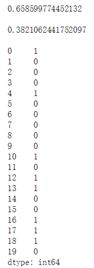

from sklearn.linear_model import LogisticRegression
from sklearn.model_selection import cross_val_predict
"""
权重项可以自己定义的
0代表5倍的
1代表10倍的
"""
penalty = {
    0: 5,
    1: 1
}

lr = LogisticRegression(class_weight=penalty)
# kf = KFold(features.shape[0], random_state=1)
kf = 10
predictions = cross_val_predict(lr, features, target, cv=kf)
predictions = pd.Series(predictions)

# False positives.
fp_filter = (predictions == 1) & (loans["loan_status"] == 0)
fp = len(predictions[fp_filter])

# True positives.
tp_filter = (predictions == 1) & (loans["loan_status"] == 1)
tp = len(predictions[tp_filter])

# False negatives.
fn_filter = (predictions == 0) & (loans["loan_status"] == 1)
fn = len(predictions[fn_filter])

# True negatives
tn_filter = (predictions == 0) & (loans["loan_status"] == 0)
tn = len(predictions[tn_filter])

# Rates
tpr = tp / float((tp + fn))
fpr = fp / float((fp + tn))

print(tpr)
print()
print(fpr)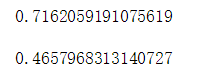

那么为什么会出现上面极其离谱的现象呢？这是由于我们的样本是很不均衡的，这就容易导致我们构建的分类器把所有样本都归为样本量较大的那一个类。解决的方法有很多，其中一个是进行数据增强，就是把少的样本增多，但是要添加的数据要么是收集的，要么是自己造的，所以这项工作还是挺难的。所以将考虑权重，将少的样本的权重增大，期望模型能够达到比较均衡的状态。

对上述模型的预测结果进行简单的分析，发现错误率和正确率都达到99.9%，错误率太高，通过观察预测结果发现，模型几乎将所有的样本都判断为正例，通过对原始数据的了解，分析造成该现象的原因是由于政府样本数量相差太大，即样本不均衡造成模型对正例样本有所偏重，这里采用对样本添加权重值的方式进行调整，首先采用默认的均衡调整。

以上案例不是着重给出一个正确率的预测模型，只是给出使用机器学习建模的一般流程，分为两大部分：数据处理和模型学习，第一部分需要大量的街舞知识对原始数据进行清理及特征提取，第二部分模型学习，涉及长时间的模型参数调整，调整方向和策略需要大家进一步的研究。模型效果不理想时，可以考虑的调整策略：

1.调节正负样本的权重参数。

2.更换模型算法。

3.同时几个使用模型进行预测，然后取去测的最终结果。

4.使用原数据，生成新特征。

5.调整模型参数

数据分析痴迷者

关注

1
点赞
踩
17

收藏

觉得还不错? 一键收藏
0
评论
python之客户逾期还款业务

数据源结构：数据集是Lending Club平台发生借贷的业务数据，共有52个变量，39522条记录。1、数据预处理去掉一些明显没用的特征。import pandas as pdimport numpy as npimport matplotlib.pyplot as pltimport seaborn as snsimport warningswarnings....
复制链接

扫一扫