tensorflow使用sequential实现简单线性回归

tensorflow使用sequential实现简单线性回归

sequential介绍

sequential理解为堆叠，通过堆叠许多层，构建出深度神经网络

https://tensorflow.google.cn/api_docs/python/tf/keras/Sequential

获取或生成csv文件

1. 生成大致符合y = 2*x + 5的一组数据，并加入噪声
2. 写入文件，需要注意第一次写入和追加写入

import csv
import numpy as np
import matplotlib.pyplot as plt
import os

# 生成x值
x = np.random.randint(1, 101, size=100)

# 生成带有一些噪声的y值，修改scale值增加噪声偏差
y = 2*x + 5 + np.random.normal(scale=0.2, size=len(x))

# 添加额外的20%噪声（生成多次，其中一次加入大噪声）
y += np.random.normal(scale=0.2*np.abs(y), size=len(y))

# 保留2位小数
x = np.round(x, 2)
y = np.round(y, 2)

# 如果data.csv不存在，则创建文件并写入表头
if not os.path.exists('data.csv'):
    with open('data.csv', mode='w') as file:
        writer = csv.writer(file)
        writer.writerow(['x', 'y'])
        for i in range(len(x)):
            writer.writerow([x[i], y[i]])

# 如果data.csv存在，则使用追加写入模式
else:
    with open('data.csv', mode='r') as file:
        reader = csv.reader(file)
        header = next(reader)
        if header != ['x', 'y']:
            raise ValueError("The header of data.csv is not correct.")
    with open('data.csv', mode='a') as file:
        writer = csv.writer(file)
        for i in range(len(x)):
            writer.writerow([x[i], y[i]])

print("数据已写入data.csv")

plt.scatter(x, y)
plt.show()

分别修改参数，为了拟合的准确性

线性回归实现

1.读取包含线性关系的.csv文件

data = pd.read_csv('./data.csv')
print(data)

2.将数据划分为训练集和测试集

train_data = data.sample(frac=0.8, random_state=0)
test_data = data.drop(train_data.index)

3.顺序模型squential的建立

顺序模型是指网络是一层一层搭建的，前面一层的输出是后一层的输入，采用线性激活的全连接(Dense)层，它实际上封装了输入值x乘以权重w，加上偏置(bias)b，然后进行线性激活以产生输出

model = tf.keras.Sequential()
model.add(tf.keras.layers.Dense(1, input_shape=(1,)))

4.查看模型的结构

model.summary()

5.编译模型

配置的过程, 优化算法方式（梯度下降）、损失函数选择mse即均方误差，Adam优化器的学习速率默认为0.01

model.compile(optimizer='adam', loss='mse')

6.训练模型

记录模型的训练过程 history，如果模型存在，则加载模型继续训练
训练过程是loss函数值降低的过程，即不断逼近最优的a和b参数值的过程，这个过程要训练很多次epoch，epoch是指对所有训练数据训练的次数

if os.path.exists('./model.h5'):
    model = tf.keras.models.load_model('./model.h5')

history = model.fit(train_data.x, train_data.y, epochs=1000)
model.save('./model.h5')

7.评估模型

accuracy = model.evaluate(test_data.x, test_data.y)
print("Accuracy: {:.2f}%".format(accuracy * 100))

8.已知数据预测

model.predict(test_data.x)
print(model.predict(test_data.x))

9.随机数据预测

test_predict = model.predict(pd.Series([10, 20]))  # 预测的数据为10和20
print(test_predict)
print(pd.DataFrame([(10, 20, 30)]))

10.绘制训练过程的loss

plt.plot(history.history['loss'])
plt.title('Model Loss')
plt.ylabel('Loss')
plt.xlabel('Epoch')
plt.show()

11 查看权重和偏移

res = model.layers[0].get_weights()
w = res[0][0][0]
b = res[1][0]
print(w)
print(b)

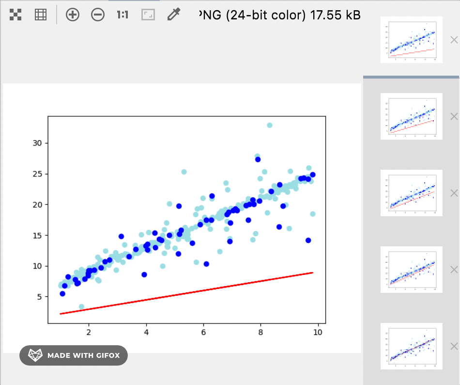
12 将训练集，测试集和最后的训练结果绘制到图上

plt.plot(data.x, w * data.x + b, color='red')
plt.scatter(train_data.x, train_data.y, color='powderblue')
plt.scatter(test_data.x, test_data.y, color='blue')
plt.show()

训练过程和结果

// step 8
[[25.062683]
 [45.056755]]

// step 9
    0   1   2
0  10  20  30

// step 11
1.9994073
5.06861