Iris Classification 鸢尾花分类

一、 简介

根据鸢尾花的四个特征萼片长度（ Sepal length）, 萼片宽度（Sepal width）, 花瓣长度（Petal length）, 花瓣宽度（Petal width），区分鸢尾花的三个品种山鸢尾（Iris-setosa）、变色鸢尾（Iris-versicolor）和维吉尼亚鸢尾（Iris-virginica）。实现基础的三分类问题

二、数据集

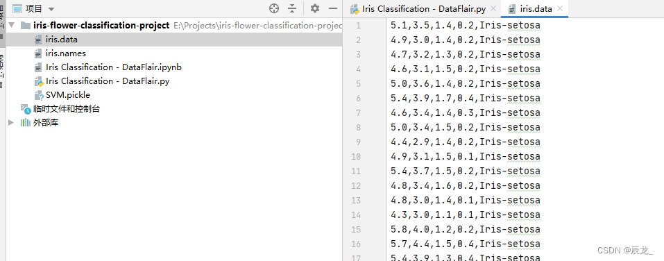
一共150行，每行由5个数据，分别是四个特征和鸢尾花品种

三、代码解读

引入库

import numpy as np
import matplotlib.pyplot as plt
import seaborn as sns
import pandas as pd

columns = ['Sepal length', 'Sepal width', 'Petal length', 'Petal width', 'Class_labels'] 

读取数据集并显示基本情况

df = pd.read_csv('iris.data', names=columns)
df.head()
df.describe()

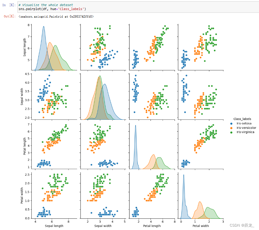
可视化整个数据集

sns.pairplot(df, hue='Class_labels')

将特征和标签分离

data = df.values
X = data[:,0:4]
Y = data[:,4]

计算三个类别的每个特征的平均值

Y_Data = np.array([np.average(X[:, i][Y==j].astype('float32')) for i in range (X.shape[1]) for j in (np.unique(Y))])

查看Y_Data

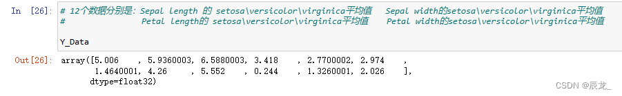
重塑，变为三行四列的矩阵。第一行代表山鸢尾（Iris-setosa）品种的4个特征，第二行代表变色鸢尾（Iris-versicolor）的4个特征，第三行代表维吉尼亚鸢尾（Iris-virginica）品种的4个特征

Y_Data_reshaped = Y_Data.reshape(4, 3)
Y_Data_reshaped = np.swapaxes(Y_Data_reshaped, 0, 1)

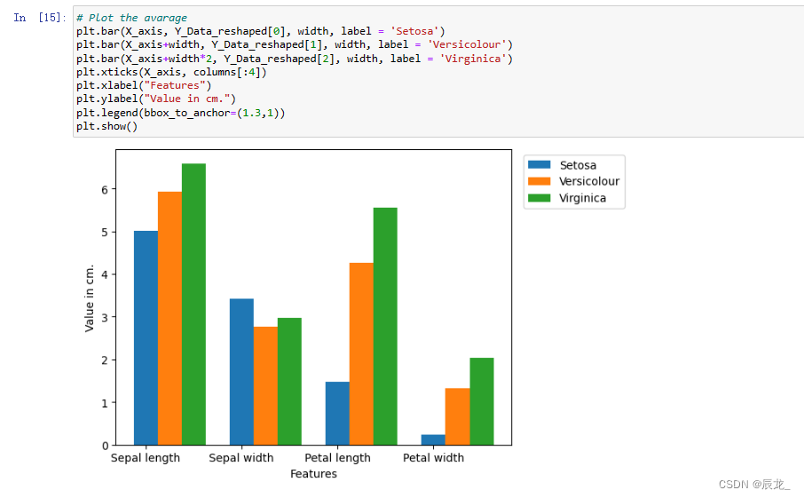
绘制图像

X_axis = np.arange(len(columns)-1)
width = 0.25
plt.bar(X_axis, Y_Data_reshaped[0], width, label = 'Setosa')
plt.bar(X_axis+width, Y_Data_reshaped[1], width, label = 'Versicolour')
plt.bar(X_axis+width*2, Y_Data_reshaped[2], width, label = 'Virginica')
plt.xticks(X_axis, columns[:4])
plt.xlabel("Features")
plt.ylabel("Value in cm.")
plt.legend(bbox_to_anchor=(1.3,1))
plt.show()

分割测试集和数据集

from sklearn.model_selection import train_test_split
X_train, X_test, y_train, y_test = train_test_split(X, Y, test_size=0.2)

使用训练集 X_train 和对应的类别标签 y_train 对支持向量机分类器进行训练。fit 方法会根据提供的训练数据学习出一个决策边界，以便将不同类别的样本正确分类。

from sklearn.svm import SVC
svn = SVC()
svn.fit(X_train, y_train)

# 预测测试集
predictions = svn.predict(X_test)

# 计算准确率
from sklearn.metrics import accuracy_score
accuracy_score(y_test, predictions)

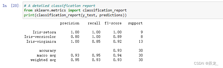
生成详细报告

from sklearn.metrics import classification_report
print(classification_report(y_test, predictions))

自己编写3组数据（每组包含4个特征值），进行测试

X_new = np.array([[3, 2, 1, 0.2], [  4.9, 2.2, 3.8, 1.1 ], [  5.3, 2.5, 4.6, 1.9 ]])
prediction = svn.predict(X_new)
print("Prediction of Species: {}".format(prediction))

保存模型和加载模型

import pickle
with open('SVM.pickle', 'wb') as f:
    pickle.dump(svn, f)
# with open('SVM.pickle', 'wb') as f:: 使用 open 函数以二进制写入模式打开一个文件 'SVM.pickle'，
# 这里指定了文件名和打开模式。'wb' 表示以二进制写入模式打开文件，如果文件不存在，则创建该文件；如果文件已存在，则覆盖原有内容

# 尝试使用先前的模型进行训练
with open('SVM.pickle', 'rb') as f:
    model = pickle.load(f)
    model.predict(X_new)

四、 完整代码

# DataFlair Iris Classification
# Import Packages
import numpy as np
import matplotlib.pyplot as plt
import seaborn as sns
import pandas as pd

columns = ['Sepal length', 'Sepal width', 'Petal length', 'Petal width', 'Class_labels'] 
# As per the iris dataset information

# Load the data
df = pd.read_csv('iris.data', names=columns)
df.head()
# Some basic statistical analysis about the data
df.describe()

# Visualize the whole dataset
sns.pairplot(df, hue='Class_labels')

# Seperate features and target  
data = df.values
X = data[:,0:4]
Y = data[:,4]

# Calculate avarage of each features for all classes
Y_Data = np.array([np.average(X[:, i][Y==j].astype('float32')) for i in range (X.shape[1]) for j in (np.unique(Y))])
Y_Data_reshaped = Y_Data.reshape(4, 3)
Y_Data_reshaped = np.swapaxes(Y_Data_reshaped, 0, 1)
X_axis = np.arange(len(columns)-1)
width = 0.25

# Plot the avarage
plt.bar(X_axis, Y_Data_reshaped[0], width, label = 'Setosa')
plt.bar(X_axis+width, Y_Data_reshaped[1], width, label = 'Versicolour')
plt.bar(X_axis+width*2, Y_Data_reshaped[2], width, label = 'Virginica')
plt.xticks(X_axis, columns[:4])
plt.xlabel("Features")
plt.ylabel("Value in cm.")
plt.legend(bbox_to_anchor=(1.3,1))
plt.show()

# Split the data to train and test dataset.
from sklearn.model_selection import train_test_split
X_train, X_test, y_train, y_test = train_test_split(X, Y, test_size=0.2)

# Support vector machine algorithm
from sklearn.svm import SVC
svn = SVC()
svn.fit(X_train, y_train)

# Predict from the test dataset
predictions = svn.predict(X_test)

# Calculate the accuracy
from sklearn.metrics import accuracy_score
accuracy_score(y_test, predictions)

# A detailed classification report
from sklearn.metrics import classification_report
print(classification_report(y_test, predictions))
X_new = np.array([[3, 2, 1, 0.2], [  4.9, 2.2, 3.8, 1.1 ], [  5.3, 2.5, 4.6, 1.9 ]])

#Prediction of the species from the input vector
prediction = svn.predict(X_new)
print("Prediction of Species: {}".format(prediction))

# Save the model
import pickle
with open('SVM.pickle', 'wb') as f:
    pickle.dump(svn, f)
    
# Load the model
with open('SVM.pickle', 'rb') as f:
    model = pickle.load(f)
model.predict(X_new)