TensorFlow上手（一）

深度学习领域的计算机实现最常用的两个工具包是Tensorflow和Pytorch。因此，有必要对这两个工具包的一些操作使用方法做一些简介。我们先从TensorFlow开始吧，安装很简单，直接pip即可：

pip install tensorflow

张量

• 张量

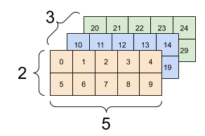
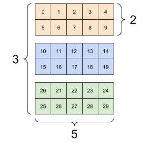
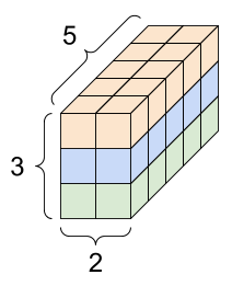
tf最底层的数组被称为张量，跟numy的array是等价的，比如创建一个形状为[3,2,5]的张量,利用tf的constan方法即可：

# There can be an arbitrary number of
# axes (sometimes called "dimensions")
rank_3_tensor = tf.constant([
  [[0, 1, 2, 3, 4],
   [5, 6, 7, 8, 9]],
  [[10, 11, 12, 13, 14],
   [15, 16, 17, 18, 19]],
  [[20, 21, 22, 23, 24],
   [25, 26, 27, 28, 29]],])

print(rank_3_tensor)

它的展现形式可以多种多样：

tf的张量可以转换为numpy形式：

np.array(tf_tensor)
tf_tensor.numpy()

• 运算
  

张量可以进行运算，常用的有相加，相乘以及矩阵相乘：

a = tf.constant([[1, 2],[3, 4]])
b = tf.constant([[1, 1],[1, 1]]) # Could have also said `tf.ones([2,2])`

print(tf.add(a, b), "\n") #对应位置相加,相当a+b
print(tf.multiply(a, b), "\n") #对应位置相乘,相当a*b
print(tf.matmul(a, b), "\n") #矩阵相乘,相当a@b

也可以进行一些复杂运算：

c = tf.constant([[4.0, 5.0], [10.0, 1.0]])

print(tf.reduce_max(c)) # 最大的值
print(tf.argmax(c)) # 每行坐标值最大的索引
print(tf.nn.softmax(c)) # Compute the softmax

• 形状
  

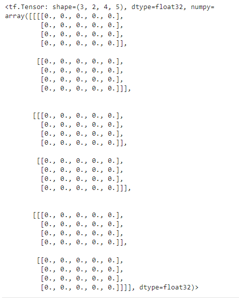
张量的形状很重要，它是规定传入数据的维度、规模，比如下面具有4个维度的张量：

rank_4_tensor = tf.zeros([3, 2, 4, 5])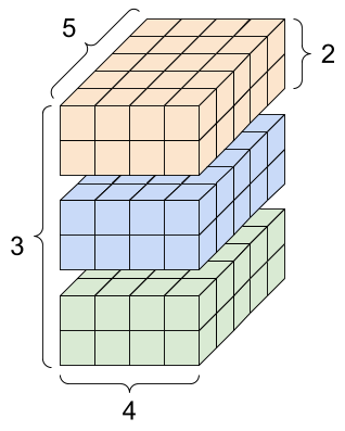

它的输出如下：

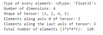
我们可以打印其各种属性：

print("Type of every element:", rank_4_tensor.dtype)
print("Number of dimensions:", rank_4_tensor.ndim)
print("Shape of tensor:", rank_4_tensor.shape)
print("Elements along axis 0 of tensor:", rank_4_tensor.shape[0])
print("Elements along the last axis of tensor:", rank_4_tensor.shape[-1])
print("Total number of elements (3*2*4*5): ", tf.size(rank_4_tensor).numpy())

结果如下：

• 索引

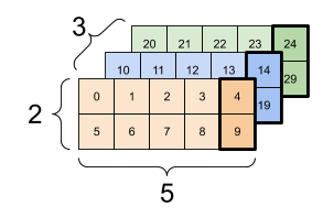
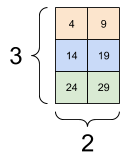
张量的索引与切片遵循python从0开始的原则，与numpy几乎无差异，这里只说一个例子。对于形状为[3,2,5]的张量，每个示例最后一个特征的代码为：

tf_tensor[:, :, 4]

                                   

• 重构
  

重构数据类型可以使用cast()方法：

the_f64_tensor = tf.constant([2.2, 3.3, 4.4], dtype=tf.float64)
the_f16_tensor = tf.cast(the_f64_tensor, dtype=tf.float16)
the_u8_tensor = tf.cast(the_f16_tensor, dtype=tf.uint8)

形状可以变为列表：

var_x = tf.Variable(tf.constant([[1], [2], [3]]))
var_x.shape.as_list()

可以重新定义形状大小：

reshaped = tf.reshape(var_x, [1, 3])
tf.reshape(rank_3_tensor, [-1])# 变为一行
tf.reshape(rank_3_tensor, [3*2, 5]) #指定形状

• 其他

也可以定义不规则张量和稀疏张量

ragged_list = [[0, 1, 2, 3],[4, 5],[6, 7, 8],[9]]
ragged_tensor = tf.ragged.constant(ragged_list)

sparse_tensor = tf.sparse.SparseTensor(
            indices=[[0, 0], [1, 2]],
                values=[1, 2],
            dense_shape=[3, 4])

tf.sparse.to_dense(sparse_tensor)

自动微分

深度学习领域，反向传播中需要计算梯度，因此，tensorflow提供了一种叫梯度带的东西来记录变量的梯度变化过程。

首先，要定义变量，通过tf.Variable实现：

my_tensor = tf.constant([[1.0, 2.0], [3.0, 4.0]])
my_variable = tf.Variable(my_tensor)

# Variables can be all kinds of types, just like tensors
bool_variable = tf.Variable([False, False, False, True])
complex_variable = tf.Variable([5 + 4j, 6 + 1j])

变量可以转换为张量，但它无法重构形状，直接指定重构的话，会变成张量：

print("A variable:",my_variable)
print("\nViewed as a tensor:", tf.convert_to_tensor(my_variable))
print("\nIndex of highest value:", tf.argmax(my_variable))

# This creates a new tensor; it does not reshape the variable.
print("\nCopying and reshaping: ", tf.reshape(my_variable, ([1,4])))

变量可以进行命名，并且，指定它是否需要进行微分：

a = tf.Variable(my_tensor, name="Mark")
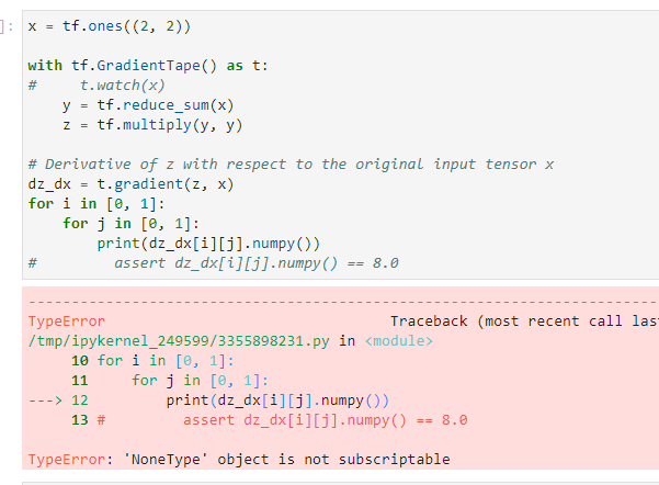
step_counter = tf.Variable(1, trainable=False)

通常情况下，如果要监视的是一个张量，通过watch方法进行监视：

x = tf.ones((2, 2))

with tf.GradientTape() as t:
    t.watch(x)
    y = tf.reduce_sum(x)
    z = tf.multiply(y, y)

# Derivative of z with respect to the original input tensor x
dz_dx = t.gradient(z, x)
for i in [0, 1]:
    for j in [0, 1]:
        print(dz_dx[i][j].numpy())

这里，x是一个张量，通过梯度带Gradient.Tape()来监视它，使得它可以对z=z(x)进行求微分。如果不进行监视，则报错：

默认情况下,调用一次GradientTape.gradient()后，其占用的内存资源会被是否，无法进行多次调用，如果要对同一个函数对多个变量求导，则需要声明persistent为True：

x = tf.constant(3.0)
with tf.GradientTape(persistent=True) as t:
    t.watch(x)
    y = x * x
    z = y * y
dz_dx = t.gradient(z, x) # 108.0 (4*x^3 at x = 3)
dy_dx = t.gradient(y, x) # 6.0

用多个梯度带则可以进行高阶导数，比如二次导：

x = tf.Variable(1.0) # Create a Tensorflow variable initialized to 1.0

with tf.GradientTape() as t:
    with tf.GradientTape() as t2:
        y = x * x * x
        
# Compute the gradient inside the 't' context manager
# which means the gradient computation is differentiable as well.
    dy_dx = t2.gradient(y, x)
d2y_dx2 = t.gradient(dy_dx, x)

assert dy_dx.numpy() == 3.0
assert d2y_dx2.numpy() == 6.0

认识tf.Module

• 指定可训练参数
  

深度学习一般都是由层组成，因此，tensorflow的实现模型都是基于tf.Module构建。

我们先简单认识一下这个基类都有些什么基础属性：

class SimpleModule(tf.Module):
    
    def __init__(self, name=None):
        
        super().__init__(name=name)
        self.a_variable = tf.Variable(5.0, name="train_me")
        self.non_trainable_variable = tf.Variable(6.0, trainable=False, name="do_not_train_me")
        
    def __call__(self, x):
        
        return self.a_variable * x + self.non_trainable_variable

上面的SimpleModule继承了tf.Module类，它初始化方法继承了tf.module的初始化方法，这个里面可以看到声明最基本的是否把某个变量作为可训练的参数：

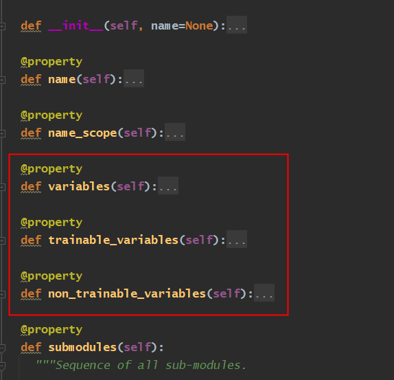
通过trainable设置为False声明为不可训练的参数，比如上面的non_trainable_variable变量，我们打印所有的变量：

Every variable
print("all variables:", simple_module.variables)

# All trainable variables
print("trainable variables:", simple_module.trainable_variables)

# All not trainable variables
print("trainable variables:", simple_module.non_trainable_variables)

• 定义层Dense
  

接下来我们通过一个最简单的例子来看看tf如何定义神经网络的层，MLP是最基本的NN模型，不妨看看两层的MLP模型：

class Dense(tf.Module):
    def __init__(self, in_features, out_features, name=None):
        super().__init__(name=name)
        self.w = tf.Variable(tf.random.normal([in_features, out_features]), name='w')
        self.b = tf.Variable(tf.zeros([out_features]), name='b')
    def __call__(self, x):
        y = tf.matmul(x, self.w) + self.b
        return tf.nn.relu(y)

首先，这是每层的初始化权重，系数w是服从正态分布的，偏移系数b均为0，然后通过relu激活函数输出。

class SequentialModule(tf.Module):
    def __init__(self, name=None):
        
        super().__init__(name=name)
        self.dense_1 = Dense(in_features=3, out_features=3)
        self.dense_2 = Dense(in_features=3, out_features=2)

    def __call__(self, x):
        x = self.dense_1(x)
        return self.dense_2(x)

然后，定义了两层MLP，第一层输入是3个神经元，下一层也是3个神经元，输出是2层。只要调用SequentialModule的call方法就可以得到最后的输出层结果。

这里需要指定下一层的神经元个数，实际上可以做到可变的，根据输入来调整：

class FlexibleDenseModule(tf.Module):
  # Note: No need for `in+features`
    def __init__(self, out_features, name=None):
        super().__init__(name=name)
        self.is_built = False
        self.out_features = out_features

    def __call__(self, x):
        # Create variables on first call.
        if not self.is_built:
            self.w = tf.Variable(tf.random.normal([x.shape[-1], self.out_features]), name='w')
            self.b = tf.Variable(tf.zeros([self.out_features]), name='b')
            self.is_built = True

        y = tf.matmul(x, self.w) + self.b
        return tf.nn.relu(y)


# Used in a module
class MySequentialModule(tf.Module):
    def __init__(self, name=None):
        
        super().__init__(name=name)
        self.dense_1 = FlexibleDenseModule(out_features=3)
        self.dense_2 = FlexibleDenseModule(out_features=2)

    def __call__(self, x):
        x = self.dense_1(x)
        return self.dense_2(x)

认识Keras

• keras.layer.Layer
  

tf有一个包Keras,它也是一个实现与tf相同功能的更简单的包,它的基类是keras.layer.Layer，继承tf.Module，下面是定义层的例子：

class MyDense(tf.keras.layers.Layer):
    # Adding **kwargs to support base Keras layer arguemnts
    def __init__(self, in_features, out_features, **kwargs):
        super().__init__(**kwargs)

        # This will soon move to the build step; see below
        self.w = tf.Variable(tf.random.normal([in_features, out_features]), name='w')
        self.b = tf.Variable(tf.zeros([out_features]), name='b')
        
    def call(self, x):
        y = tf.matmul(x, self.w) + self.b
        return tf.nn.relu(y)

simple_layer = MyDense(name="simple", in_features=3, out_features=3)
simple_layer([[2.0, 2.0, 2.0]])

• build函数
  

输入层也可以在给定向量后再生成，用build函数，只不过仅被调用一次，而且是使用输入的形状调用的。

class FlexibleDense(tf.keras.layers.Layer):
    # Note the added `**kwargs`, as Keras supports many arguments
    def __init__(self, out_features, **kwargs):
        super().__init__(**kwargs)
        self.out_features = out_features

    def build(self, input_shape): # Create the state of the layer (weights)
        self.w = tf.Variable(tf.random.normal([input_shape[-1], self.out_features]), name='w')
        self.b = tf.Variable(tf.zeros([self.out_features]), name='b')

    def call(self, inputs): # Defines the computation from inputs to outputs
        return tf.matmul(inputs, self.w) + self.b

• keras.Model
  
  

keras.Model提供了全功能模型，它继承了keras.layer.Layer，利用它可以定义多层模型：

class MySequentialModel(tf.keras.Model):
    def __init__(self, name=None, **kwargs):
        super().__init__(**kwargs)

        self.dense_1 = FlexibleDense(out_features=3)
        self.dense_2 = FlexibleDense(out_features=2)
        
    def call(self, x):
        x = self.dense_1(x)
        return self.dense_2(x)

比如输入一个3维的向量，其输出结果是：

# You have made a Keras model!
my_sequential_model = MySequentialModel(name="the_model")
# Call it on a tensor, with random results
print("Model results:", my_sequential_model(tf.constant([[2.0, 2.0, 2.0]])))

上面两行代码运行调用时，首先初始化类MySequentialModel的初始化方法__init__()给对象my_sequential_model，这期间会调用类FlexibleDense初始化输出层的神经元个数，这里一共初始化两层，第一层神经元个数是3，第二层是2。然后，执行my_sequential_model的call方法，传入向量，这期间遇到一开始初始化的层dense_1和dense_2，会分别执行build函数和FlexibleDense的call函数，完成初始化过程。

• 函数式 API 

构造上面一样的模型，也可以使用keras的函数式API：

inputs = tf.keras.Input(shape=[3,])
x = FlexibleDense(3)(inputs)
x = FlexibleDense(2)(x)

my_functional_model = tf.keras.Model(inputs=inputs, outputs=x)
my_functional_model.summary()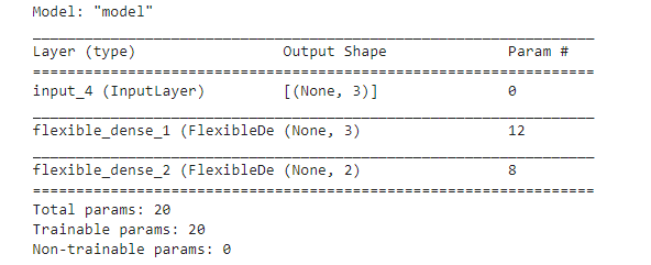

参考资料：

https://keras.io/zh/

https://tensorflow.google.cn/guide/tensor