


这篇博客主要是总结一下sklearn中给出的几种PCA方法的实现,包括
- PCA:针对线性可分数据的PCA方法的实现
- Kernel PCA:加入了核函数的PCA方法,用于对线性不可分数据的降维
- Incremental PCA:用于对大数据进行降维,当数据量过大时,不能一次全部加载入内存,所以需要每次加载一个batch,这一点上和深度学习在数据量过大时的加载方法是一致的,即每次都只从外存中取一个batch进内存进行训练。
- Sparse PCA:稀疏PCA的实现(这一块没看的太懂,就先不写了)
PCA
在sklearn中实现PCA的类为sklearn.decomposition.PCA,类的定义如下:
class sklearn.decomposition.PCA(n_components=None,
                                copy=True,
                                whiten=False,
                                svd_solver='auto',
                                tol=0.0,
                                iterated_power='auto',
                                random_state=None)
类的常用属性:
components_:array, shape (n_components, n_features),返回的是根据特征值进行排序后的主成分对应的特征向量explained_variance_:array, shape (n_components,),返回的n个主成分的方差值explained_variance_ratio_:array, shape (n_components,),返回n个主成分的方差值分别占所有方差值之和的比例singular_values_:array, shape (n_components,),返回每个主成分对应的奇异值mean_:array, shape (n_features,),返回每一维的平均值n_components_:int,返回当前PCA实例中设定的主成分个数n_features_:int,训练数据中的特征数n_samples_:int,训练数据中的样本数
类的常用方法:
fit(self, X[, y]):对原始数据进行训练,返回训练后的实例transform(self, X):对输入的X矩阵进行降维fit_transform(self, X[,y]):对原始数据进行训练并降维,返回降维后的新数据get_covariance(self):得到原始数据的协方差矩阵get_params(self, deep=True):得到当前PCA实例的参数,返回的是一个字典类型set_params(self, *params):设置当前PCA实例的参数inverse_transform(self, X):将输入的X转换会原始数据集对应的空间,即对该函数返回的矩阵做相同的降维操作能得到矩阵Xscore(self, X, y=None):返回所有样本的平均对数似然值score_samples(self, X):返回每个样本的对数似然值
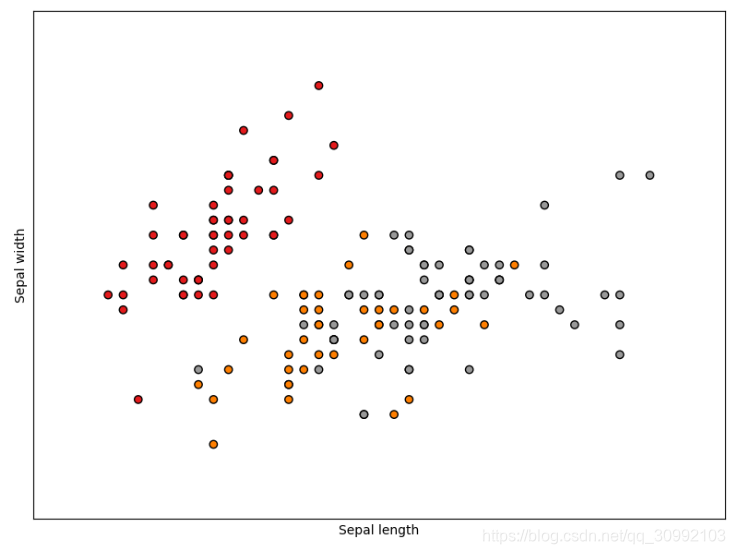
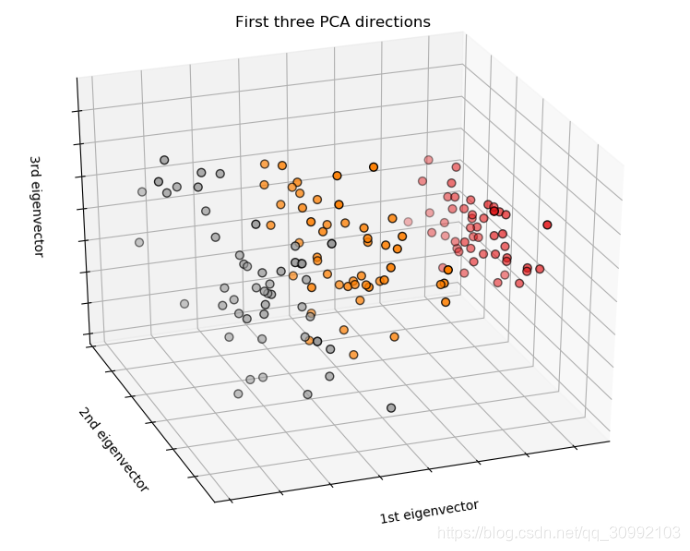
利用PCA方法对鸢尾花数据集进行降维的实例代码如下:
import matplotlib.pyplot as plt
from mpl_toolkits.mplot3d import Axes3D
from sklearn import datasets
from sklearn.decomposition import PCA

# import some data to play with
iris = datasets.load_iris()
X = iris.data[:, :2]  # we only take the first two features.
y = iris.target

x_min, x_max = X[:, 0].min() - .5, X[:, 0].max() + .5
y_min, y_max = X[:, 1].min() - .5, X[:, 1].max() + .5

plt.figure(2, figsize=(8, 6))
plt.clf()

# Plot the training points
plt.scatter(X[:, 0], X[:, 1], c=y, cmap=plt.cm.Set1,
            edgecolor='k')
plt.xlabel('Sepal length')
plt.ylabel('Sepal width')

plt.xlim(x_min, x_max)
plt.ylim(y_min, y_max)
plt.xticks(())
plt.yticks(())

# To getter a better understanding of interaction of the dimensions
# plot the first three PCA dimensions
fig = plt.figure(1, figsize=(8, 6))
ax = Axes3D(fig, elev=-150, azim=110)
pca = PCA(n_components=3)
X_reduced = pca.fit_transform(iris.data)
ax.scatter(X_reduced[:, 0], X_reduced[:, 1], X_reduced[:, 2], c=y,
           cmap=plt.cm.Set1, edgecolor='k', s=40)
ax.set_title("First three PCA directions")
ax.set_xlabel("1st eigenvector")
ax.w_xaxis.set_ticklabels([])
ax.set_ylabel("2nd eigenvector")
ax.w_yaxis.set_ticklabels([])
ax.set_zlabel("3rd eigenvector")
ax.w_zaxis.set_ticklabels([])

plt.show()
输出的结果如下:
Kernel PCA
在sklearn中实现Kernel PCA的类为sklearn.decomposition.KernelPCA,类的定义如下:
class sklearn.decomposition.KernelPCA(n_components=None,
                                      kernel='linear',
                                      gamma=None,
                                      degree=3,
                                      coef0=1,
                                      kernel_params=None,
                                      alpha=1.0,
                                      fit_inverse_transform=False,
                                      eigen_solver='auto',
                                      tol=0,
                                      max_iter=None,
                                      remove_zero_eig=False,
                                      random_state=None,
                                      copy_X=True,
                                      n_jobs=None)
其中主要需要指定的参数有主成分数目、采用的核函数和核函数的相关参数,关于核函数的内容可以参考Pairwise metrics, Affinities and Kernels
其中给定的方法包括:
fit(self, X[, y]):对原始数据进行训练,返回训练后的实例transform(self, X):对输入的X矩阵进行降维fit_transform(self, X[,y]):对原始数据进行训练并降维,返回降维后的新数据get_params(self, deep=True):得到当前PCA实例的参数,返回的是一个字典类型set_params(self, *params):设置当前PCA实例的参数inverse_transform(self, X):将输入的X转换会原始数据集对应的空间,即对该函数返回的矩阵
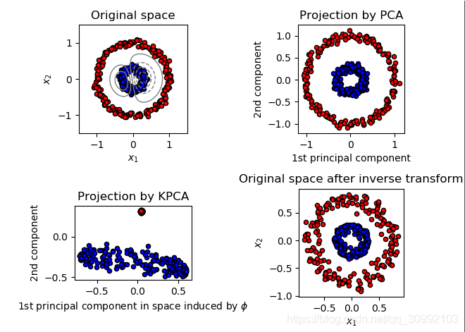
利用Kernel PCA方法对线性不可分数据进行降维的实例代码如下:
import numpy as np
import matplotlib.pyplot as plt

from sklearn.decomposition import PCA, KernelPCA
from sklearn.datasets import make_circles

np.random.seed(0)

X, y = make_circles(n_samples=400, factor=.3, noise=.05)

kpca = KernelPCA(kernel="rbf", fit_inverse_transform=True, gamma=10)
X_kpca = kpca.fit_transform(X)
X_back = kpca.inverse_transform(X_kpca)
pca = PCA()
X_pca = pca.fit_transform(X)

# Plot results

plt.figure()
plt.subplot(2, 2, 1, aspect='equal')
plt.title("Original space")
print(y)
reds = y == 0
blues = y == 1
print(reds)
print(X[reds, 0])
plt.scatter(X[reds, 0], X[reds, 1], c="red",
            s=20, edgecolor='k')
plt.scatter(X[blues, 0], X[blues, 1], c="blue",
            s=20, edgecolor='k')
plt.xlabel("$x_1$")
plt.ylabel("$x_2$")

X1, X2 = np.meshgrid(np.linspace(-1.5, 1.5, 50), np.linspace(-1.5, 1.5, 50))
X_grid = np.array([np.ravel(X1), np.ravel(X2)]).T
# projection on the first principal component (in the phi space)
Z_grid = kpca.transform(X_grid)[:, 0].reshape(X1.shape)
plt.contour(X1, X2, Z_grid, colors='grey', linewidths=1, origin='lower')

plt.subplot(2, 2, 2, aspect='equal')
plt.scatter(X_pca[reds, 0], X_pca[reds, 1], c="red",
            s=20, edgecolor='k')
plt.scatter(X_pca[blues, 0], X_pca[blues, 1], c="blue",
            s=20, edgecolor='k')
plt.title("Projection by PCA")
plt.xlabel("1st principal component")
plt.ylabel("2nd component")

plt.subplot(2, 2, 3, aspect='equal')
plt.scatter(X_kpca[reds, 0], X_kpca[reds, 1], c="red",
            s=20, edgecolor='k')
plt.scatter(X_kpca[blues, 0], X_kpca[blues, 1], c="blue",
            s=20, edgecolor='k')
plt.title("Projection by KPCA")
plt.xlabel(r"1st principal component in space induced by $\phi$")
plt.ylabel("2nd component")

plt.subplot(2, 2, 4, aspect='equal')
plt.scatter(X_back[reds, 0], X_back[reds, 1], c="red",
            s=20, edgecolor='k')
plt.scatter(X_back[blues, 0], X_back[blues, 1], c="blue",
            s=20, edgecolor='k')
plt.title("Original space after inverse transform")
plt.xlabel("$x_1$")
plt.ylabel("$x_2$")

plt.tight_layout()
plt.show()
得到的结果如下图所示:
Incremental PCA
增量PCA在sklearn中的实现的类为class sklearn.decomposition.IncrementalPCA,类的定义为:
class sklearn.decomposition.IncrementalPCA(n_components=None,
                                           whiten=False,
                                           copy=True,
                                           batch_size=None)
其中参数batch_size用于设置每次加载的batch的大小。
类的属性包括:
components_:array, shape (n_components, n_features),返回的是根据方差进行排序后的主成分对应的特征向量explained_variance_:array, shape (n_components,),返回的n个主成分的方差值explained_variance_ratio_:array, shape (n_components,),返回n个主成分的方差值分别占所有方差值之和的比例singular_values_:array, shape (n_components,),返回每个主成分对应的奇异值mean_:array, shape (n_features,),当前已经训练过的所有样本的每一维特征的平均值var_:array, shape (n_features,),当前已经训练过的所有样本的每一维特征的方差值n_components_:int,返回当前PCA实例中设定的主成分个数n_features_:int,训练数据中的特征数n_samples_seen_:int,当前已经被训练过的样本数
类的方法包括:
fit(self, X[, y]):对原始数据进行训练,返回训练后的实例transform(self, X):对输入的X矩阵进行降维fit_transform(self, X[,y]):对原始数据进行训练并降维,返回降维后的新数据get_covariance(self):得到原始数据的协方差矩阵get_params(self, deep=True):得到当前PCA实例的参数,返回的是一个字典类型set_params(self, *params):设置当前PCA实例的参数inverse_transform(self, X):将输入的X转换会原始数据集对应的空间,即对该函数返回的矩阵做相同的降维操作能得到矩阵Xpartial_fit(self, X[,y,check_input]):利用输入的样本集X进行增量训练
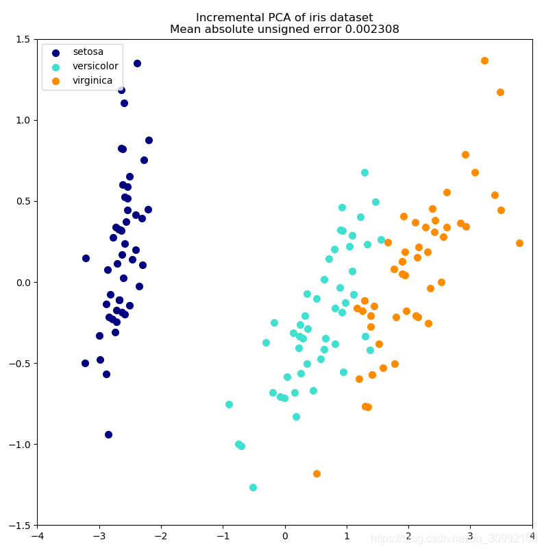
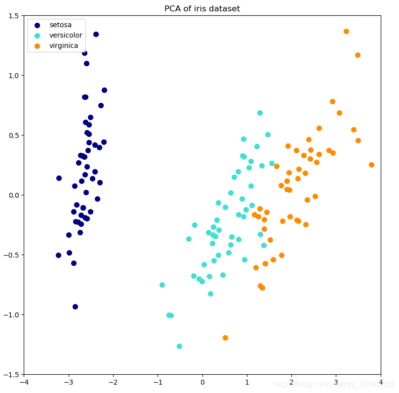
利用增量PCA对鸢尾花数据集进行降维的实例如下,同时将增量PCA的结果与用传统线性PCA进行降维的结果进行对比:
import numpy as np
import matplotlib.pyplot as plt

from sklearn.datasets import load_iris
from sklearn.decomposition import PCA, IncrementalPCA

iris = load_iris()
X = iris.data
y = iris.target

n_components = 2
ipca = IncrementalPCA(n_components=n_components, batch_size=10)
X_ipca = ipca.fit_transform(X)

pca = PCA(n_components=n_components)
X_pca = pca.fit_transform(X)

colors = ['navy', 'turquoise', 'darkorange']

for X_transformed, title in [(X_ipca, "Incremental PCA"), (X_pca, "PCA")]:
    plt.figure(figsize=(8, 8))
    for color, i, target_name in zip(colors, [0, 1, 2], iris.target_names):
        plt.scatter(X_transformed[y == i, 0], X_transformed[y == i, 1],
                    color=color, lw=2, label=target_name)

    if "Incremental" in title:
        err = np.abs(np.abs(X_pca) - np.abs(X_ipca)).mean()
        plt.title(title + " of iris dataset\nMean absolute unsigned error "
                  "%.6f" % err)
    else:
        plt.title(title + " of iris dataset")
    plt.legend(loc="best", shadow=False, scatterpoints=1)
    plt.axis([-4, 4, -1.5, 1.5])

plt.show()
代码输出为:


 被折叠的 条评论
为什么被折叠?
被折叠的 条评论
为什么被折叠?
 到【灌水乐园】发言


