


转自:https://blog.csdn.net/Dorisi_H_n_q/article/details/82313244,进行了整理结合
其他常用的统计方法有:
常用统计方法
count 非 NA 值的数量
describe 针对 Series 或 DF 的列计算汇总统计
min , max 最小值和最大值
argmin , argmax 最小值和最大值的索引位置(整数)
idxmin , idxmax 最小值和最大值的索引值
quantile 样本分位数(0 到 1)
sum 求和
mean 均值
median 中位数
mad 根据均值计算平均绝对离差
var 方差
std 标准差
skew 样本值的偏度(三阶矩)
kurt 样本值的峰度(四阶矩)
cumsum 样本值的累计和
cummin , cummax 样本值的累计最大值和累计最小值
cumprod 样本值的累计积
diff 计算一阶差分(对时间序列很有用)
pct_change 计算百分数变化
1、删除重复元素
使用duplicated()函数检测重复的行,返回元素为布尔类型的Series对象,每个元素对应一行,如果该行不是第一次出现,则元素为True
-
import numpy
as np
-
import pandas
as pd
-
from pandas
import Series,DataFrame
-
-
import matplotlib.pyplot
as plt
-
%matplotlib inline
-
创建数据集:
-
# color 0 :red;1:green;2:blue
-
df = DataFrame({
'color':np.random.randint(
0,
3,size =
300),
'num':np.random.randint(
0,
5,size =
300)})
-
df
-
-
#或者:
-
b=np.random.choice([
'B',
'M'],size=(
100,
2))
-
b1=DataFrame(b,columns=[
'True',
'Predict'])
-
b1


-
# 计算True的总个数,即计算重复的总行数
-
df.duplicated().sum()
-
Out:
285
-
使用drop_duplicates()函数删除重复的行【inplace=True则会修改原数组】
df.drop_duplicates()

- 查看图片中的重复元素
-
img = plt.imread(
'./芝麻.jpg')
-
img.shape
-
Out: (
662,
1000,
3)
-
-
# 这张图片总共有多少个像素呢?
-
# (红,绿,蓝)
-
662*
1000
-
Out:
662000
-
-
# numpy没有去重的方法
-
img2 = img.reshape(
-1,
3)
-
img2
-
# img2 必须是转化成n行n列,比如reshape(-1,3)
-
df = DataFrame(img2,columns=[
'red',
'green',
'blue'])
-
df
-
-
# 总数据662000
-
# 非重复的像素,71526个 ,inplace=True则能修改原数组
-
df.drop_duplicates().shape
-
Out: (
71526,
3)
【注意】如果使用pd.concat([df1,df2],axis = 1)生成新的DataFrame,新的df中columns相同,使用duplicate()和drop_duplicates()都会出问题
2. 映射
映射的含义:创建一个映射关系列表,把values元素和一个特定的标签或者字符串绑定
需要使用字典:
map = { 'label1':'value1', 'label2':'value2', ... }
包含三种操作:
- replace()函数:替换元素
- 最重要:map()函数:新建一列
- rename()函数:替换索引
1) replace()函数:替换元素
使用replace()函数,对values进行替换操作
- 定义数据集
-
df = DataFrame({
'color':np.random.randint(
0,
3,size =
300),
'num':np.random.randint(
10,
30,size =
300)})
-
df

- 首先定义一个字典
m = {0:'red',1:'green',2:'blue'}
- 调用.replace()
-
# replace方法,可将DataFrame中所有满足条件的数据,进行替换
-
df.replace(m)

- replace还经常用来替换NaN元素
-
# 字典的key类型要一致
-
m = {
0:
'red',
1:
'green',
2:
'blue',
1024:
'purple',
2048:
'cyan'}
-
-
# 字典中映射关系,键值对,去DataFrame找数据,找到了就替换,没有找到,也不会报错
-
df.replace(m)
- 使用正则匹配替换:
数据集 data1 ——> 杂质:-数字\t

法①:遍历—> re.sub
-
import re
-
data1[
0].map(
lambda x: re.sub(
'.*\d+\\t',
'',x))
法②【一定要加上.str才能替换】:data1[0].str.replace
pd.DataFrame(data1[0].str.replace('.*?\d+?\\t ', '')) #用正则表达式修改数据
2) map()函数:新建一列
使用map()函数,由已有的列生成一个新列
适合处理某一单独的列。
仍然是新建一个字典
map()函数中可以使用lambda函数
transform()和map()类似
使用map()函数新建一个新列
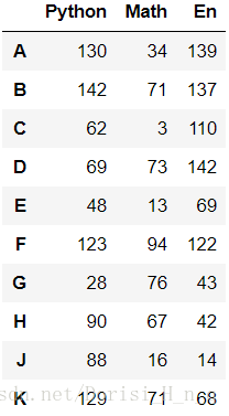
- 新建数据集
-
df = DataFrame(np.random.randint(
0,
150,size = (
10,
3)),
-
columns=[
'Python',
'Math',
'En'],index=list(
'ABCDEFGHJK'))
-
df
- map映射简单lambda函数
-
# df['Python'] 10 个数据 迭代器
-
df[
'Java'] = df[
'Python'].map(
lambda x :
2*x -
100)
-
df

-
f =
lambda x : x*
2 -
100
-
type(f)
-
Out: function
-
-
def fun(x):
-
x*
2 -
100
-
type(fun)
-
Out: function
- 定义一个函数level,带入map函数:
-
def convert(x):
-
if x >=
130:
-
return
'优秀'
-
elif x <
130
and x >=
100:
-
return
'良好'
-
elif x <
100
and x >=
80:
-
return
'中等'
-
elif x <
80
and x >=
60:
-
return
'及格'
-
else:
-
return
'不及格'
-
-
df[
'Level'] = df[
'Python'].map(convert)
-
df

- 给某一列都加上某个数:法① df['Python'] += 10
-
# Python 这一列,老师出考题的时候,有一道题出错了,每个人Python加10分
-
df[
'Python'] +=
10
-
df

- 给某一列都加上某个数:法② map(lambda x : x+10)
-
# map 这个方法,可以修改当前的列
-
df[
'Python'] = df[
'Python'].map(
lambda x :x +
10)
-
df
- 分箱操作:
分箱、分块、分类——》
# 分箱,分类
# 葡萄品质0~10
# 0~4 low
# 5~7 median
# 8~10 high
-
# 分箱,分类
-
# 葡萄品质0~10
-
# 0~4 low
-
# 5~7 median
-
# 8~10 high
-
-
# 0 ~ 10 信用
-
# 0~3 low
-
# 4~ 6 median
-
# 7~10 high
-
-
# 根据这个人手机产生数据
-
def convert(x):
-
if x >=
140:
-
return
150
-
elif x <
140
and x >=
100:
-
return
125
-
elif x <
100
and x>=
60:
-
return
80
-
else:
-
return
0
-
-
df[
'Python'] = df[
'Python'].map(convert)
-
df

3) rename()函数:替换索引
- 新建数据集:
-
df = DataFrame(np.random.randint(
0,
150,size = (
4,
3)))
-
df

- 仍然是新建一个字典,使用rename()函数替换行索引
-
# 更改列标题 【axis = 0 行】
-
m = {
0:
'张三',
1:
'李四',
2:
'王五',
3:
'小刘'}
-
df.rename(m,axis =
0,inplace=
True)
-
-
# 更改行标题
-
m = {
0:
'Python',
1:
'Math',
2:
'En'}
-
df.rename(m,axis =
1,inplace=
True)
-
df

3. 异常值检测和过滤
使用describe()函数查看每一列的描述性统计量
- 新建数据集
-
df = DataFrame(np.random.randn(
10000,
3),columns=list(
'ABC'))
-
df

- 检测异常值:① 求出每一列均值;② 异常值判断条件:大于5倍均值
-
# 过滤条件,大于5倍平均,异常
-
# 均值0.79,则大于3.95为异常值
-
df.abs().mean()
-
Out:
-
A
0.798357
-
B
0.793909
-
C
0.789348
-
dtype: float64
-
-
# 找出各个属性的异常值
-
cond = df.abs() >
3.95
-
cond.sum()
-
Out:
-
A
2
-
B
2
-
C
0
-
dtype: int64
-
-
# 异常值总和
-
(cond.sum()).sum()
-
-
# 异常值总行数
-
cond.any(axis =
1).sum()
-
Out:
4
-
-
# 以DataFrame形式展示存在异常值的行数
-
df[cond.any(axis =
1)]

展示满足要求的数据:
-
# 满足要求的数据
-
cond = df.abs() <=
3.95
-
cond = cond.all(axis =
1)
-
df[cond]

- 使用std()函数可以求得DataFrame对象每一列的标准差;
- 根据每一列的标准差,对DataFrame元素进行过滤;
- 借助any()函数, 测试是否有True,有一个或以上返回True,反之返回False;
- 对每一列应用筛选条件,去除标准差太大的数据
3原则:如果数据服从正态分布,在3原则下,异常值被定义为一组测定值中与平均值的偏差超过3倍标准差的值。在正态分布的假设下,距离平均值3之外的值出现的概率为P(|x-|>3)≤0.003,属于极个别的小概率事件。
-
#平均值上下三倍标准差之间属于正常点
-
std=df.abs().std()
-
std
-
Out:
-
A
0.607076
-
B
0.598781
-
C
0.594652
-
dtype: float64
-
-
mean=df.abs().mean()
-
mean
-
Out:
-
A
0.798357
-
B
0.793909
-
C
0.789348
-
dtype: float64
-
-
low=mean
-3*std
-
high=mean+
3*std
-
display(low.mean(),high.mean())
-
Out:
-
-1.0066372280404017
-
2.5943795581659246
-
-
# 异常值 位于小于mean-3*std or 大于mean+3*std
-
low1=df.abs()<low.mean()
-
high1=df.abs() > high.mean()
-
low_high1=np.logical_or(low1,high1)
-
low_high1
-
-
# 显示异常值个数
-
df[low_high1.any(axis=
1)].shape
-
Out: (
259,
3)
-
# 过滤掉正常值,显示异常值
-
df[low_high1.any(axis=
1)]
-
-
#平均值上下三倍标准差之间属于正常点
-
lowcond=df.abs()>low.mean()
-
highcond=df.abs() < high.mean()
-
low_high=np.logical_and(lowcond,highcond)
-
low_high
-
-
# 过滤异常值,满足条件 df.mean()-3*df.std() ~ df.mean()+3*df.std()
-
df[low_high.all(axis=
1)].shape
-
Out: (
9741,
3)
-
-
df.shape
-
Out:(
10000,
3)
-
259+
9741=
10000
- 新建数据集:身高、体重
- 手动创建异常值
- 判定异常值范围
- 过滤异常值
-
df =DataFrame(
-
{
'height':np.random.randint(
150,
200,
1000),
-
'weight':np.random.randint(
50,
90,size =
1000)})
-
df
-
-
# 创造异常值
-
# 每隔10个数据加一个300,比如第10个原本63,处理后变363,第20,30..一样
-
df[
'weight'][::
10] +
300
-
df
-
-
# 判定异常值范围:
-
# 体重的异常值:>300公斤
-
cond = df[
'weight'] <
300
-
-
# 异常值筛选:给定条件(数据不同,条件不一样,根据数据属性来做选择)
-
df[cond]
4. 排序及打乱下标随机排序
使用.take()函数排序,可以借助np.random.permutation()函数随机排序
df.take([100,300,210])

-
# 产生5个0-4的随机数
-
np.random.permutation(
5)
-
Out: array([
2,
0,
4,
3,
1])
-
-
# 产生1000个0-999的随机数
-
index = np.random.permutation(
1000)
-
index
-
type(index)
-
Out: numpy.ndarray
-
-
# 使用产生的随机数作为下标排序显示数据
-
df.take(index)
- 另一种产生n个 0 ~ n-1 的随机数
-
# 产生1000个从0~999的升序数列
-
index = np.arange(
1000)
-
index
-
-
# 打乱0~999的顺序数列
-
np.random.shuffle(index)
-
index
-
display(type(index),index)
-
Out: numpy.ndarray
-
-
# 使用随机打乱的数列作为下标显示数据
-
df.take(index)
随机抽样
当DataFrame规模足够大时,直接使用np.random.randint()函数,就配合take()函数实现随机抽样
-
df = DataFrame(np.random.randn(
10000,
3),columns=list(
'ABC'))
-
df
-
-
df.size
-
Out:
30000

-
ss=np.random.randint(
0,
10000,size =
100)
-
ss
-
Out:
-
array([
4065,
9998,
4088,
2039,
4184,
1807,
1325,
1569,
6657,
2974,
3211,
-
2982,
8154,
7668,
6738,
7486,
4362,
105,
6373,
3119,
1261,
1648,
-
2962,
7112,
2243,
6014,
2211,
6357,
2032,
1761,
7664,
6734,
1882,
-
6126,
8942,
4872,
8935,
9207,
4533,
4558,
9922,
5127,
9340,
5148,
-
640,
8374,
5681,
1160,
325,
2469,
9823,
7114,
8228,
5019,
4217,
-
2901,
8420,
4888,
4274,
6595,
2289,
1446,
8035,
958,
736,
7005,
-
5490,
2752,
3260,
9686,
5241,
3165,
8381,
7885,
4582,
8015,
7215,
-
8430,
8921,
4957,
2419,
7912,
9510,
1614,
1102,
3070,
2390,
228,
-
3588,
829,
6808,
4883,
349,
1869,
2073,
1992,
9280,
1085,
5495,
-
5396])
-
-
DataFrame(ss)[
0].unique().size
-
Out:
100
-
-
# 可以直接使用random.randint 产生的数据来做下标随机抽取数据
-
df.take(np.random.randint(
0,
10000,size =
100))
5. 数据聚合【重点】
数据聚合是数据处理的最后一步,通常是要使每一个数组生成一个单一的数值。
数据分类处理:
- 分组:先把数据分为几组
- 用函数处理:为不同组的数据应用不同的函数以转换数据
- 合并:把不同组得到的结果合并起来
数据分类处理的核心: groupby()函数
- 创建数据集
-
df = DataFrame({
'item':np.random.randint(
0,
4,
50),
-
'level':np.random.randint(
0,
3,size =
50),
-
'price':np.random.randint(
1,
10,size =
50),
-
'sailer':np.random.randint(
0,
3,size =
50),
-
'weight':np.random.randint(
50,
100,size =
50)})
-
df

- 赋值转换
-
# = 赋值 :使用map({字典集})
-
df[
'item'] = df[
'item'].map({
0:
'萝卜',
1:
'白菜',
2:
'西红柿',
3:
'黄瓜'})
-
df[
'level'] = df[
'level'].map({
0:
'差',
1:
'中',
2:
'优'})
-
df[
'sailer'] = df[
'sailer'].map({
0:
'张大妈',
1:
'李大妈',
2:
'赵大叔'})
-
df

- 聚合操作
-
# 按 sailer,item分组,显示价格的最大值
-
aa=df.groupby([
'sailer',
'item'])[
'price'].max()
-
aa
-
-
Out:[Series]
-
sailer item
-
张大妈 白菜
8
-
萝卜
8
-
西红柿
9
-
黄瓜
2
-
李大妈 白菜
4
-
萝卜
6
-
西红柿
7
-
黄瓜
9
-
赵大叔 白菜
8
-
萝卜
9
-
西红柿
8
-
黄瓜
8
-
Name: price, dtype: int32
-
-
# 按等级,类别分组,显示价格和体重的最小值
-
df.groupby([
'level',
'item'])[
'price',
'weight'].min()

- 求总和
-
weight_sum = df.groupby([
'level'])[
'weight'].sum()
-
weight_sum
-
Out:
-
level
-
中
1570
-
优
790
-
差
1250
-
Name: weight, dtype: int64

-
# 给表头修改名字
-
weight_sum = weight_sum.rename({
'weight':
'weight_sum'},axis =
1)
-
weight_sum

- 合并聚合表格【左连接:left_on='level',right_index=True】注意:没有right_index=True会报错
-
df2 = df.merge(weight_sum,left_on=
'level',right_index=
True)
-
df2

- 求平均价格
-
price_mean = df.groupby([
'item'])[
'price'].mean()
-
price_mean = DataFrame(price_mean)
-
price_mean
-
-
# 修改标题名称
-
price_mean.columns = [
'price_mean']
-
price_mean

- 合并聚合数据表格
df2.merge(price_mean,left_on='item',right_index=True)

============================================
练习23:
- 假设菜市场张大妈在卖菜,有以下属性:
- 菜品(item):萝卜,白菜,辣椒,冬瓜
- 颜色(color):白,青,红
- 重量(weight)
- 价格(price)
- 要求以属性作为列索引,新建一个ddd
- 对ddd进行聚合操作,求出颜色为白色的价格总和
- 对ddd进行聚合操作,求出萝卜的所有重量(包括白萝卜,胡萝卜,青萝卜)以及平均价格
- 使用merge合并总重量及平均价格
============================================
-
# 测试choice
-
np.random.choice([
0,
1,
2],size=
10)
-
Out:
-
array([
1,
0,
1,
1,
0,
2,
2,
1,
2,
2])
- 创建数据集
-
ddd=DataFrame({
'item':np.random.choice([
'萝卜',
'白菜',
'辣椒',
'冬瓜'],size=
50),
-
'color':np.random.choice([
'白',
'青',
'红'],size=
50),
-
'weight':np.random.randint(
10,
100,
50),
-
'price':np.random.randint(
1,
10,
50)
-
})
-
ddd

- 求出颜色为白色的价格总和
-
ddd.color.map(
lambda x:x==
'白').sum()
-
Out:
19
- 对ddd进行聚合操作,求出萝卜的所有重量(包括白萝卜,胡萝卜,青萝卜)以及平均价格
-
p=ddd.groupby(
'item')[
'price'].mean()
-
p=DataFrame(p)
-
p
-
-
p.index
-
Out: Index([
'冬瓜',
'白菜',
'萝卜',
'辣椒'], dtype=
'object', name=
'item')
-
-
p.columns
-
Out: Index([
'price'], dtype=
'object')
-
-
w=ddd.groupby(
'item')[
'weight'].sum()
-
w=DataFrame(w)
-
w

- 使用merge合并总重量及平均价格
p.merge(w,left_index=True,right_index=True)

p.join(w)

============================================
6.0 高级数据聚合
可以使用pd.merge()函数将聚合操作的计算结果添加到df的每一行
使用groupby分组后调用加和等函数进行运算,让后最后可以调用add_prefix(),来修改列名
可以使用transform和apply实现相同功能
在transform或者apply中传入函数即可
- 采用上面的数据集

- 使用apply
df.groupby(['sailer','item'])['price'].apply(np.mean)

- 使用transform
-
# apply和transform都可以进行分组计算,计算结果一样
-
# 表现形式不同,apply多层索引,图形直观,简洁
-
# transform 一层索引,所有的数据,级联方便
-
mean_price = df.groupby([
'sailer',
'item'])[[
'price']].transform(np.mean).add_prefix(
'mean_')
-
mean_price

- 使用pd.concat()拼接mean_price
pd.concat([df,mean_price],axis = 1)

transform()与apply()函数还能传入一个函数或者lambda
-
df = DataFrame({
'color':[
'white',
'black',
'white',
'white',
'black',
'black'],
-
'status':[
'up',
'up',
'down',
'down',
'down',
'up'],
-
'value1':[
12.33,
14.55,
22.34,
27.84,
23.40,
18.33],
-
'value2':[
11.23,
31.80,
29.99,
31.18,
18.25,
22.44]})
举栗子
-
dic = {
-
'item':[
'萝卜',
'白菜',
'萝卜',
'辣椒',
'冬瓜',
'冬瓜',
'萝卜',
'白菜'],
-
'color':[
'red',
'white',
'green',
'red',
'green',
'white',
'white',
'green'],
-
'weight':[
12,
30,
16,
5,
10,
5,
25,
18],
-
'price':[
2.5,
0.8,
3.5,
4,
1.2,
1.5,
0.9,
3]
-
}
-
df = DataFrame(data=dic)
-
df

定义函数
-
# 定义求和
-
def m_sum(items):
-
sum=
0
-
for item
in items:
-
sum+=item
-
return sum
-
-
# 定义求平均
-
def my_mean(items):
#参数为复数(List形式)
-
sum=
0
-
for item
in items:
-
sum+=item
-
return sum/items.size
-
df.groupby(by=
'item')[
'weight'].apply(m_sum)[
'萝卜']
-
Out:
-
53
-
-
df.groupby(by=
'item')[
'price'].apply(my_mean)
-
Out:
-
item
-
Apple
3.00
-
Banana
2.75
-
Orange
3.50
-
Name: price, dtype: float64


 180
180


 被折叠的 条评论
为什么被折叠?
被折叠的 条评论
为什么被折叠?
 到【灌水乐园】发言


