计算机图形图像处理 实验二

原文：http://blog.csdn.net/babygoodmorning/article/details/71138158

计算机图形图像实验

一. 图像平滑

图像平滑，主要要用到openCV里的函数cvSmooth，如下

/*
src 原图像
dst 目标图像
smoothtype 平滑类型
    CV_BLUR 均值滤波
    CV_MEDIAN 中值滤波
    CV_GAUSSIAN 高斯滤波
    CV_BILATERAL 双向滤波
size1 平滑操作，窗口的宽，必须是奇数
size2 平滑操作，窗口的宽，为0的话和size1大小相等，
sigma1 用于高斯滤波
sigma2 用于双向滤波
*/
cvSmooth(cvArr *src,cvArr *dst, int smoothtype, int size1,int size2, double sigma1,double sigma2)
 
 
1
2
3
4
5
6
7
8
9
10
11
12
13
14

1. 均值滤波

IplImage* blurSmooth(IplImage* src, int size) {
    IplImage* dst = cvCreateImage(cvSize(src->width, src->height), src->depth, src->nChannels);
    cvSmooth(src, dst, CV_BLUR, size, 0, 0, 0);
    return dst;
}
 
 
1
2
3
4
5

2. 中值滤波

/*
中值滤波
窗口的增加->图像的损坏加大
*/
IplImage* medianSmooth(IplImage* src, int size) {
    IplImage* dst = cvCreateImage(cvSize(src->width, src->height), src->depth, src->nChannels);
    cvSmooth(src, dst, CV_MEDIAN, size, 0, 0, 0);
    return dst;
}
 
 
1
2
3
4
5
6
7
8
9

3. 高斯滤波

/*
高斯滤波
抑制服从正态分布的噪声有效
g(x)=exp( -x^2/(2*(sigma^2))
*/
IplImage* gaussianSmooth(IplImage* src,int size) {

    IplImage* dst = cvCreateImage(cvSize(src->width, src->height), src->depth, src->nChannels);
    cvSmooth(src, dst, CV_GAUSSIAN, size, 0, 0, 0);
    return dst;
}
 
 
1
2
3
4
5
6
7
8
9
10
11

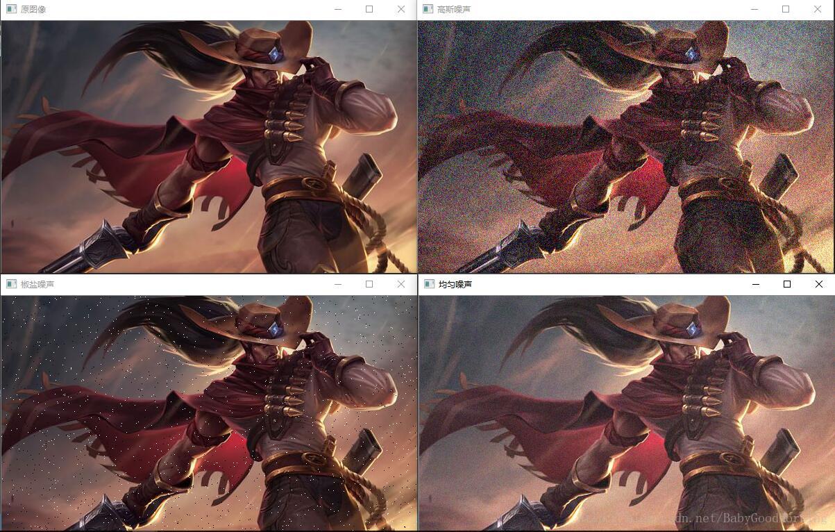
4. 实验结果

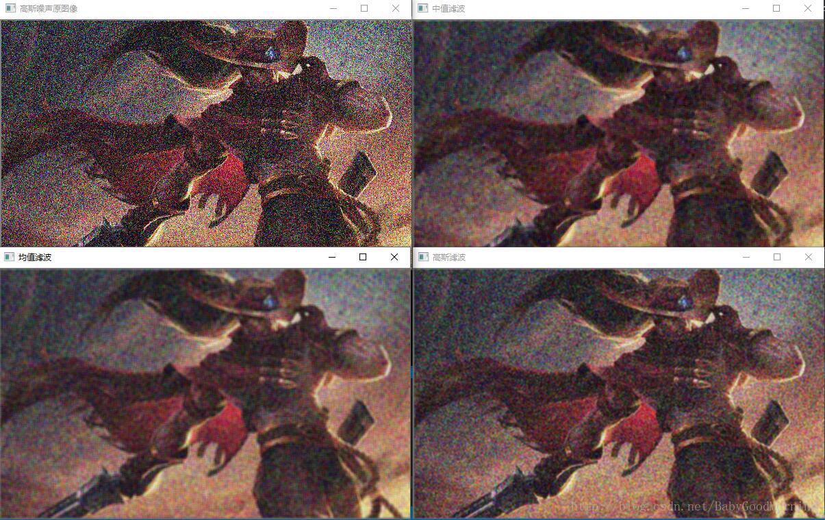
由以上结果可知，高斯滤波对于含有高斯噪声图像的处理结果较好，仔细看会发现要比均值滤波和中值滤波在细节上会更加清晰一点

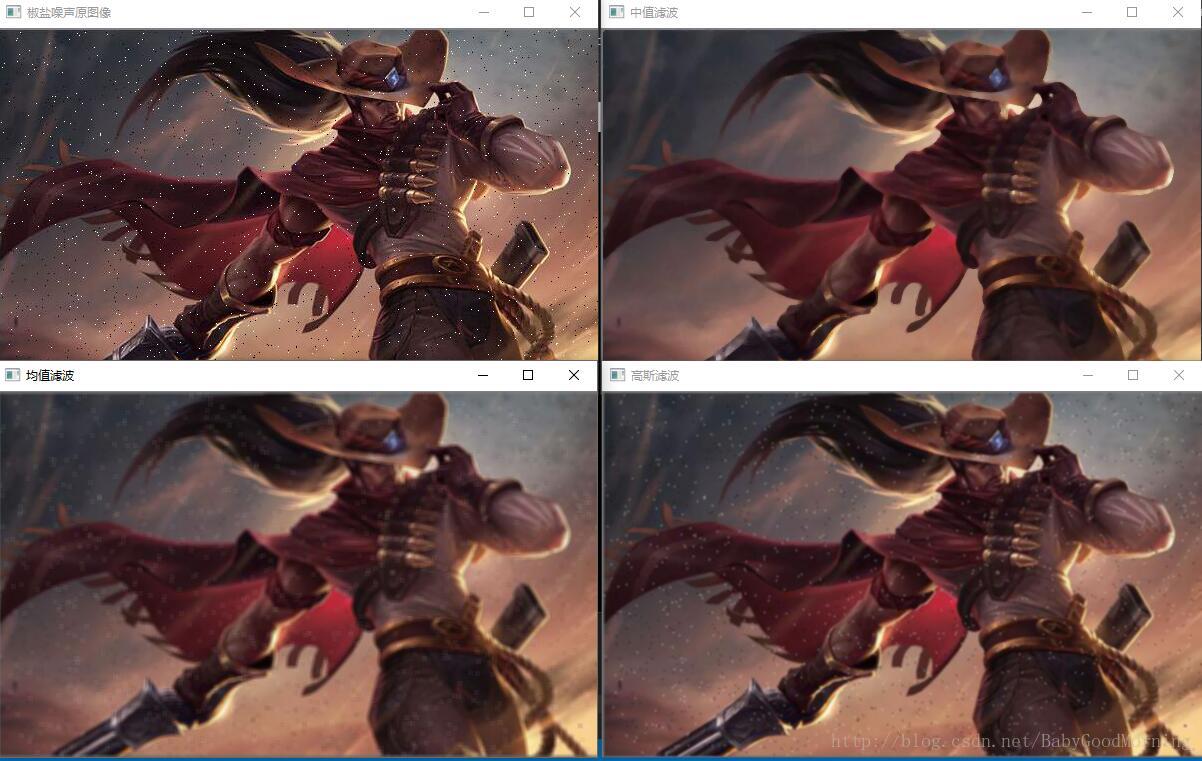
椒盐噪声图像中，带有随机分布的白点(盐)，灰点(椒)，中值滤波区中间值，能够有效过滤这两种灰度值的极值，因此，中值滤波对椒盐噪声的处理结果较好

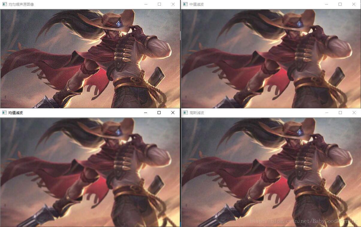
对于均匀噪声的添加是否正确，这个我不太清楚。按照自己的做法添加均匀噪声后，图像滤波如上所示，就清晰度来说还是高斯滤波的处理效果较好(仔细看可以发现的)

二. 图像锐化

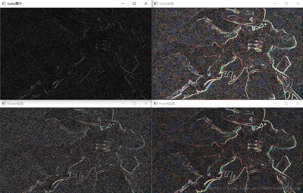
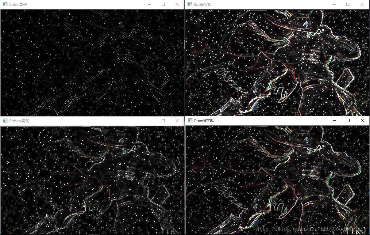
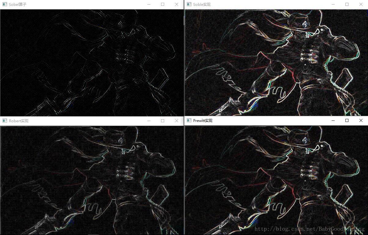
1. Sobel算子

x方向梯度算子 Gx

⎡⎣⎢10−120−210−1⎤⎦⎥

y方向梯度算子 Gy

⎡⎣⎢121000−1−2−1⎤⎦⎥

⎡⎣⎢0−1−210−1210⎤⎦⎥⎡⎣⎢−2−10−101012⎤⎦⎥

IplImage* sobelSharp(IplImage* src) { 
    IplImage* dst = cvCreateImage(cvSize(src->width, src->height), src->depth, src->nChannels);
    cvSobel(src, dst, 1, 1, 3);
    return dst;
}
 
 
1
2
3
4
5

2. Robert算子

梯度采用的是对角方向相邻两像素之差

Δxf(x,y)=f(x,y)−f(x−1,y−1)

[−11]

Δyf(x,y)=f(x−1,y)−f(x,y−1)

[1−1]

IplImage* robertSharp(IplImage* src) {
    IplImage* dst = cvCreateImage(cvSize(src->width, src->height), src->depth, src->nChannels);
    char *srcData = src->imageData;

    int width = dst->width;
    int height = dst->height;
    int widthStep = dst->widthStep;
    char *imageData = dst->imageData;

    for (int i = 1; i < height; i++) {

        uchar* curLine = (uchar*)(srcData + i * widthStep);
        uchar* preLine = curLine - widthStep;

        uchar* ptr = (uchar*)(imageData + i * widthStep);
        for (int j = 1; j < width; j++) {

            for (int rgb = 0; rgb < 3; rgb++) {
                double deltaX = curLine[3 * j + rgb] - preLine[3 * (j - 1) + rgb];
                double deltaY = curLine[3 * (j - 1) + rgb] - preLine[3 * j + rgb];
                double sum = abs(deltaX) + abs(deltaY);
                if (sum > 255) sum = 255;
                ptr[3 * j + rgb] = sum;
            }

        }

    }
    return dst;
}
 
 
1
2
3
4
5
6
7
8
9
10
11
12
13
14
15
16
17
18
19
20
21
22
23
24
25
26
27
28
29
30

3. Prewitt算子

x方向梯度算子 Gx

⎡⎣⎢−101−101−101⎤⎦⎥

y方向梯度算子 Gy

⎡⎣⎢−1−1−1000111⎤⎦⎥

⎡⎣⎢0−1−110−1110⎤⎦⎥⎡⎣⎢−1−10−101011⎤⎦⎥

IplImage* sobelSharp2(IplImage* src) {
    IplImage* dst = cvCreateImage(cvSize(src->width, src->height), src->depth, src->nChannels);
    char *srcData = src->imageData;

    int width = dst->width - 1;
    int height = dst->height - 1;
    int widthStep = dst->widthStep;
    char *imageData = dst->imageData;

    for (int i = 1; i < height; i++) {

        uchar* curLine = (uchar*)(srcData + i * widthStep);
        uchar* preLine = curLine - widthStep;
        uchar* nexLine = curLine + widthStep;
        uchar* ptr = (uchar*)(imageData + i * widthStep);
        for (int j = 1; j < width; j++) {

            for (int rgb = 0; rgb < 3; rgb++) {
                double deltaX=nexLine[3*(j-1)+rgb] + 2*nexLine[3*j+rgb] + nexLine[3*(j+1)+ rgb]
                    - preLine[3*(j-1)+rgb] -2*preLine[3*j+rgb] - preLine[3*(j+1)+rgb];

                double deltaY=preLine[3*(j+1)+rgb]+2*curLine[3*(j+1)+rgb]+nexLine[3*(j+ 1)+rgb]
                    - preLine[3*(j-1)+rgb] - 2*curLine[3*(j-1)+rgb]-nexLine[3 * (j - 1) + rgb];

                double sum = (abs(deltaX)+ abs(deltaY))/4;
                if (sum > 255) sum = 255;
                ptr[3 * j + rgb] = sum;
            }
        }
    }
    return dst;
}
 
 
1
2
3
4
5
6
7
8
9
10
11
12
13
14
15
16
17
18
19
20
21
22
23
24
25
26
27
28
29
30
31
32

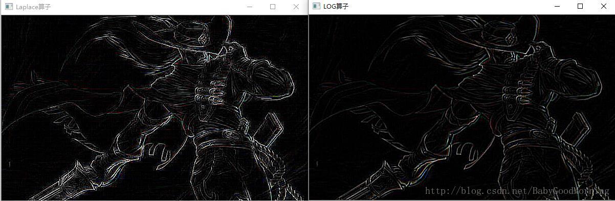
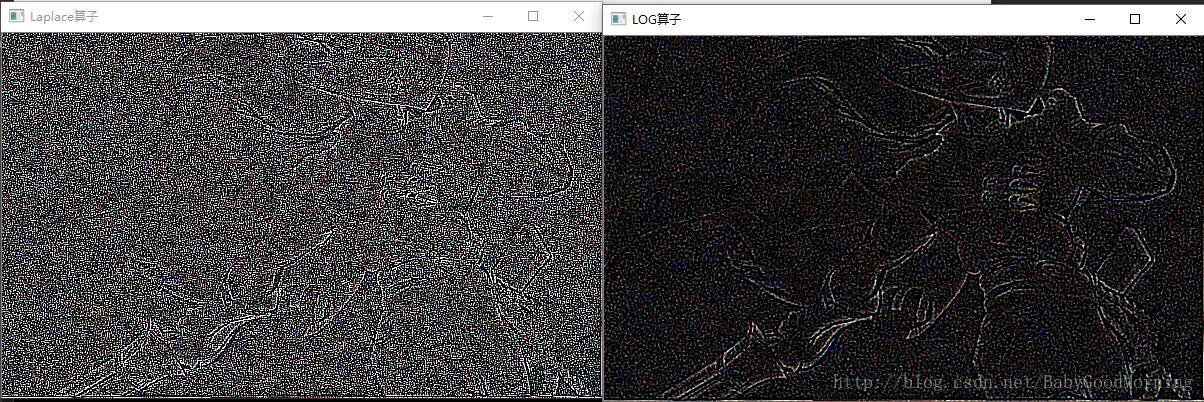
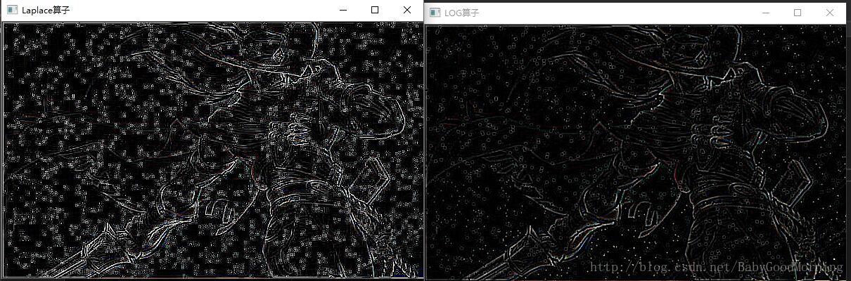
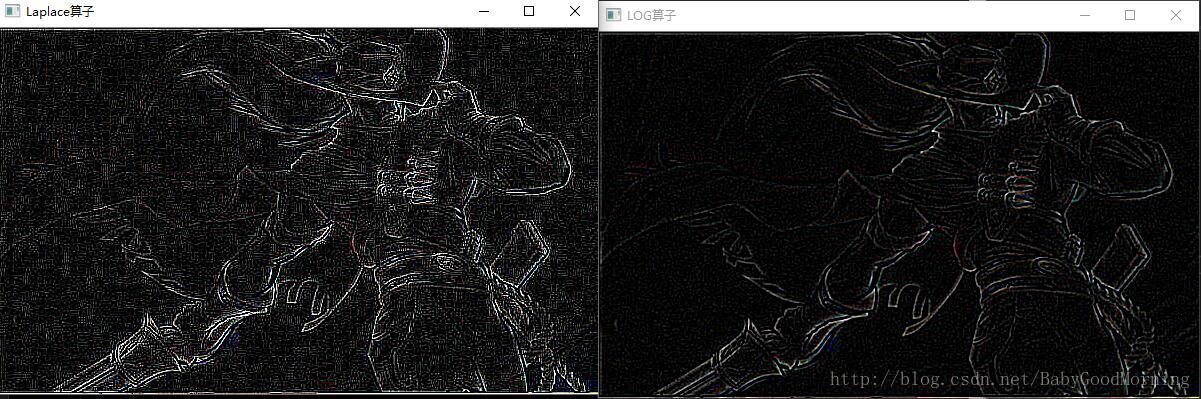
4. Laplacian算子

⎡⎣⎢0101−41010⎤⎦⎥⎡⎣⎢1111−81111⎤⎦⎥

IplImage* laplaceSharp(IplImage* src) {
    IplImage* dst = cvCreateImage(cvSize(src->width, src->height), src->depth, src->nChannels);
    cvLaplace(src, dst, 3);
    return dst;
}
 
 
1
2
3
4
5

5. LOG算子

/*
LOG算子
先使用gaussian算子 光滑滤波处理
在使用Laplace算子 进行锐化
*/

IplImage* logSharp(IplImage* src) {
    IplImage* dst = cvCreateImage(cvSize(src->width, src->height), src->depth, src->nChannels);
    cvSmooth(src, dst, CV_GAUSSIAN, 3, 0, 0, 0);
    cvLaplace(dst, dst, 3);
    return dst;
}
 
 
1
2
3
4
5
6
7
8
9
10
11
12

6. 实验结果

1. 对正常图像进行锐化

   

   

2. 对高斯噪声图像进行锐化

   

   

3. 对含有椒盐噪声的图像进行锐化

   

   

4. 对均匀噪声的图像进行锐化

   

   

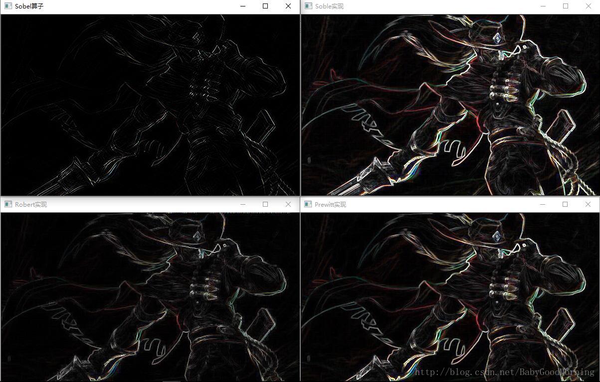
算子比较

Robert算子，边缘定位精度较高，但容易丢失一部分边缘，同时由于图像没经过平滑处理，因此不具备抑制噪声的能力。该算子对具有陡峭边缘且含噪声少的图像效果较好。

Sobel算子和Prewitt算子：都是对图像先做加权平滑处理，然后再做微分运算，所不同的是平滑部分的权值有些差异，因此对噪声具有一定的抑制能力，但不能完全排除检测结果中出现的虚假边缘。检测的边缘容易出现多像素宽度

Laplacian算子：对噪声非常敏感，它使噪声成分得到加强，这两个特性使得该算子容易丢失一部分边缘的方向信息，造成一些不连续的检测边缘，同时抗噪声能力比较差。

LOG算子：该算子首先用高斯函数对图像作平滑滤波处理，然后才使用Laplacian算子检测边缘，因此克服了Laplacian算子抗噪声能力比较差的缺点，但是在抑制噪声的同时也可能将原有的比较尖锐的边缘也平滑掉了，造成这些尖锐边缘无法被检测到。

三. 图像去噪

1. 高斯噪声

p(z)=12π√σe−(z−μ)22σ2

Z∼N[μ,σ2]

这里使用了Box-Muller转化:

假设 U1 , U2 是(0, 1)之间均匀分布的两个独立的随机变量，

Z0=Rcos(θ)=−2lnU1−−−−−−−√cos(2πU2)

Z1=Rcos(θ)=−2lnU1−−−−−−−√sin(2πU2)

则 Z0 , Z1 是两个标准正态分布的随机变量即 Z∼N[0,1]

将标准正态分布转化为非标准正态分布 F∼N[μ,σ2]

则 f=z∗σ+μ

如下转化代码摘自 https://en.wikipedia.org/wiki/Box%E2%80%93Muller_transform

(有适当改动)

double generateGaussianNoise(double mu, double sigma)
{
    const double epsilon = std::numeric_limits<double>::min();
    const double two_pi = 2.0*3.14159265358979323846;

    static double z0, z1;
    static bool generate = true;
    generate = !generate;

    if (generate)
        return z1 * sigma + mu;

    double u1, u2;
    do
    {
        u1 = rand() * (1.0 / RAND_MAX);
        u2 = rand() * (1.0 / RAND_MAX);
    } while (u1 <= epsilon);

    double sqrt_u = sqrt(-2.0 * log(u1));
    u2 *= two_pi;
    //
    z0 = sqrt_u * cos(u2);
    z1 = sqrt_u * sin(u2);
    return z0 * sigma + mu;
}
 
 
1
2
3
4
5
6
7
8
9
10
11
12
13
14
15
16
17
18
19
20
21
22
23
24
25
26

2. 椒盐噪声

salt 盐 白色，指图像中的白点，pepper胡椒 黑色 ，图像中黑色的点

/*
src 原图像
n 在图像中随机生成n个白点和黑点
*/
IplImage* saltAndPepperNoise(IplImage* src, int n) {
    IplImage* dst = src;
    int width = dst->width;
    int height = dst->height;
    int widthStep = dst->widthStep;
    char *imageData = dst->imageData;
    //添加盐噪声
    for (int i = 0; i < n; i ++) {
        int x = rand() % width;
        int y = rand() % height;
        uchar* ptr = (uchar*)(imageData + y * widthStep);
        ptr[3 * x] = 255;
        ptr[3 * x + 1] = 255;
        ptr[3 * x + 2] = 255;
    }
    //添加胡椒噪声
    for (int i = 0; i < n; i++) {
        int x = rand() % width;
        int y = rand() % height;
        uchar* ptr = (uchar*)(imageData + y * widthStep);
        ptr[3 * x] = 0;
        ptr[3 * x + 1] = 0;
        ptr[3 * x + 2] = 0;
    }
    return dst;
}
 
 
1
2
3
4
5
6
7
8
9
10
11
12
13
14
15
16
17
18
19
20
21
22
23
24
25
26
27
28
29
30

3. 均匀噪声

(0,1)的均匀分布， Z∼U[12,112],σ2=112

转化为 F∼U[μ,σ2] , 任意的均值为 μ , 方差为 σ2 的均匀分布。

f=(z−12)12−−√σ+μ

，这样可以得到我们自己想要的均匀分布

/*均匀噪声*/
IplImage* uniformNoise(IplImage* src, double mu, double sigma) {
    IplImage* dst = src;
    int width = dst->width * dst->nChannels;
    int height = dst->height;
    int widthStep = dst->widthStep;
    char *imageData = dst->imageData;

    for (int i = 0; i < height; i++) {
        uchar* ptr = (uchar*)(imageData + i * widthStep);
        for (int j = 0; j < width; j++) {
            double p1 = ptr[j] + mu + cvSqrt(12) * sigma * (rand()/(double) RAND_MAX - 0.5);
            if (p1 < 0) p1 = 0;
            if (p1 > 255) p1 = 255;
            ptr[j] = p1;
        }
    }
    return dst;
}
 
 
1
2
3
4
5
6
7
8
9
10
11
12
13
14
15
16
17
18
19

4. 实验结果

由实验结果可以得知，高斯噪声、均匀噪声，影响的是图片的没一个像素，而椒盐噪声影响的是图片的若干个点。

对于这几个图像的滤波，就不再演示了，在前面已经涉及到了。