零基础入门数据挖掘-Baseline（二手车交易价格预测）

二手车交易价格预测baseline

Tip:这是一个最初始baseline版本,抛砖引玉,为大家提供一个基本Baseline和一个竞赛流程的基本介绍，欢迎大家多多交流。

赛题：零基础入门数据挖掘 - 二手车交易价格预测

地址：https://tianchi.aliyun.com/competition/entrance/231784/introduction?spm=5176.12281957.1004.1.38b02448ausjSX

# 查看数据文件目录  list datalab files
!ls datalab/

231784

Step 1:导入函数工具箱

## 基础工具
import numpy as np
import pandas as pd
import warnings
import matplotlib
import matplotlib.pyplot as plt
import seaborn as sns
from scipy.special import jn
from IPython.display import display, clear_output
import time

warnings.filterwarnings('ignore')
%matplotlib inline

## 模型预测的
from sklearn import linear_model
from sklearn import preprocessing
from sklearn.svm import SVR
from sklearn.ensemble import RandomForestRegressor,GradientBoostingRegressor

## 数据降维处理的
from sklearn.decomposition import PCA,FastICA,FactorAnalysis,SparsePCA

import lightgbm as lgb
import xgboost as xgb

## 参数搜索和评价的
from sklearn.model_selection import GridSearchCV,cross_val_score,StratifiedKFold,train_test_split
from sklearn.metrics import mean_squared_error, mean_absolute_error

Step 2:数据读取

## 通过Pandas对于数据进行读取 (pandas是一个很友好的数据读取函数库)
Train_data = pd.read_csv('datalab/231784/used_car_train_20200313.csv', sep=' ')
TestA_data = pd.read_csv('datalab/231784/used_car_testA_20200313.csv', sep=' ')

## 输出数据的大小信息
print('Train data shape:',Train_data.shape)
print('TestA data shape:',TestA_data.shape)

Train data shape: (150000, 31)
TestA data shape: (50000, 30)

1) 数据简要浏览

## 通过.head() 简要浏览读取数据的形式
Train_data.head()

.dataframe tbody tr th {
    vertical-align: top;
}

.dataframe thead th {
    text-align: right;
}

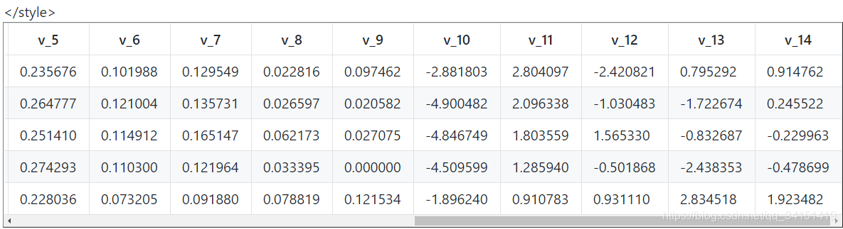
5 rows × 31 columns

2) 数据信息查看

## 通过 .info() 简要可以看到对应一些数据列名，以及NAN缺失信息
Train_data.info()

<class 'pandas.core.frame.DataFrame'>
RangeIndex: 150000 entries, 0 to 149999
Data columns (total 31 columns):
SaleID               150000 non-null int64
name                 150000 non-null int64
regDate              150000 non-null int64
model                149999 non-null float64
brand                150000 non-null int64
bodyType             145494 non-null float64
fuelType             141320 non-null float64
gearbox              144019 non-null float64
power                150000 non-null int64
kilometer            150000 non-null float64
notRepairedDamage    150000 non-null object
regionCode           150000 non-null int64
seller               150000 non-null int64
offerType            150000 non-null int64
creatDate            150000 non-null int64
price                150000 non-null int64
v_0                  150000 non-null float64
v_1                  150000 non-null float64
v_2                  150000 non-null float64
v_3                  150000 non-null float64
v_4                  150000 non-null float64
v_5                  150000 non-null float64
v_6                  150000 non-null float64
v_7                  150000 non-null float64
v_8                  150000 non-null float64
v_9                  150000 non-null float64
v_10                 150000 non-null float64
v_11                 150000 non-null float64
v_12                 150000 non-null float64
v_13                 150000 non-null float64
v_14                 150000 non-null float64
dtypes: float64(20), int64(10), object(1)
memory usage: 35.5+ MB

## 通过 .columns 查看列名
Train_data.columns

Index(['SaleID', 'name', 'regDate', 'model', 'brand', 'bodyType', 'fuelType',
       'gearbox', 'power', 'kilometer', 'notRepairedDamage', 'regionCode',
       'seller', 'offerType', 'creatDate', 'price', 'v_0', 'v_1', 'v_2', 'v_3',
       'v_4', 'v_5', 'v_6', 'v_7', 'v_8', 'v_9', 'v_10', 'v_11', 'v_12',
       'v_13', 'v_14'],
      dtype='object')

TestA_data.info()

<class 'pandas.core.frame.DataFrame'>
RangeIndex: 50000 entries, 0 to 49999
Data columns (total 30 columns):
SaleID               50000 non-null int64
name                 50000 non-null int64
regDate              50000 non-null int64
model                50000 non-null float64
brand                50000 non-null int64
bodyType             48587 non-null float64
fuelType             47107 non-null float64
gearbox              48090 non-null float64
power                50000 non-null int64
kilometer            50000 non-null float64
notRepairedDamage    50000 non-null object
regionCode           50000 non-null int64
seller               50000 non-null int64
offerType            50000 non-null int64
creatDate            50000 non-null int64
v_0                  50000 non-null float64
v_1                  50000 non-null float64
v_2                  50000 non-null float64
v_3                  50000 non-null float64
v_4                  50000 non-null float64
v_5                  50000 non-null float64
v_6                  50000 non-null float64
v_7                  50000 non-null float64
v_8                  50000 non-null float64
v_9                  50000 non-null float64
v_10                 50000 non-null float64
v_11                 50000 non-null float64
v_12                 50000 non-null float64
v_13                 50000 non-null float64
v_14                 50000 non-null float64
dtypes: float64(20), int64(9), object(1)
memory usage: 11.4+ MB

3) 数据统计信息浏览

## 通过 .describe() 可以查看数值特征列的一些统计信息
Train_data.describe()

.dataframe tbody tr th {
    vertical-align: top;
}

.dataframe thead th {
    text-align: right;
}

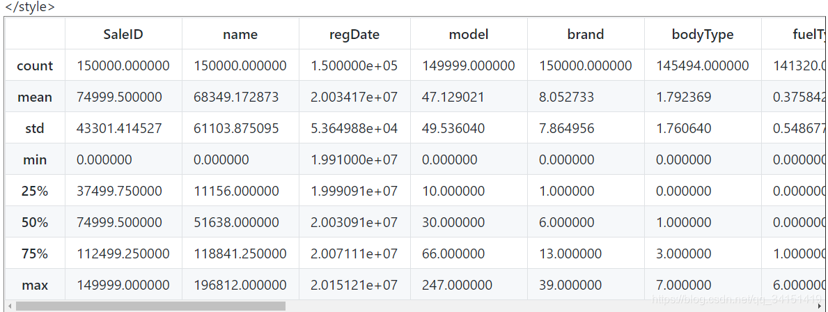
8 rows × 30 columns

TestA_data.describe()

.dataframe tbody tr th {
    vertical-align: top;
}

.dataframe thead th {
    text-align: right;
}

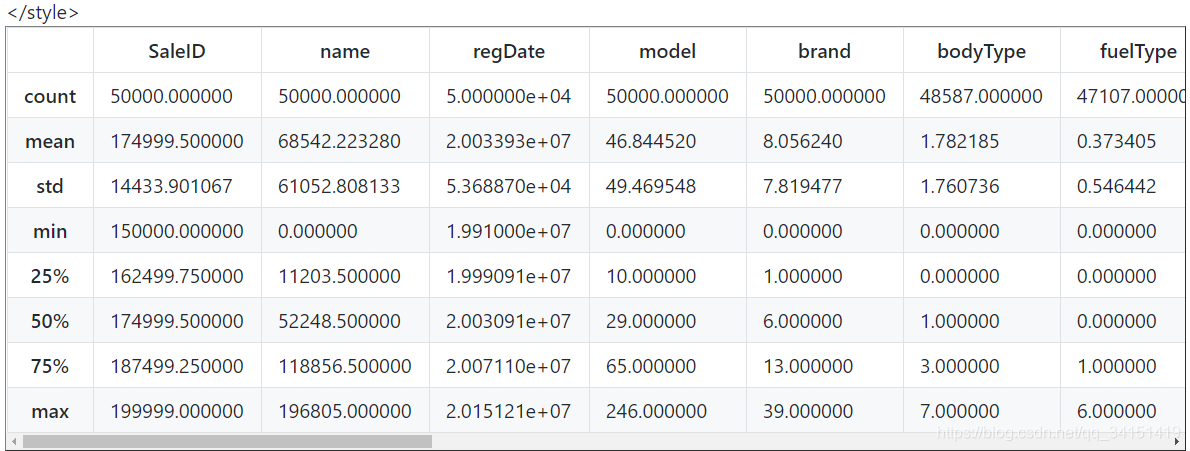
8 rows × 29 columns

Step 3:特征与标签构建

1) 提取数值类型特征列名

numerical_cols = Train_data.select_dtypes(exclude = 'object').columns
print(numerical_cols)

Index(['SaleID', 'name', 'regDate', 'model', 'brand', 'bodyType', 'fuelType',
       'gearbox', 'power', 'kilometer', 'regionCode', 'seller', 'offerType',
       'creatDate', 'price', 'v_0', 'v_1', 'v_2', 'v_3', 'v_4', 'v_5', 'v_6',
       'v_7', 'v_8', 'v_9', 'v_10', 'v_11', 'v_12', 'v_13', 'v_14'],
      dtype='object')

categorical_cols = Train_data.select_dtypes(include = 'object').columns
print(categorical_cols)

Index(['notRepairedDamage'], dtype='object')

2) 构建训练和测试样本

## 选择特征列
feature_cols = [col for col in numerical_cols if col not in ['SaleID','name','regDate','creatDate','price','model','brand','regionCode','seller']]
feature_cols = [col for col in feature_cols if 'Type' not in col]

## 提前特征列，标签列构造训练样本和测试样本
X_data = Train_data[feature_cols]
Y_data = Train_data['price']

X_test  = TestA_data[feature_cols]

print('X train shape:',X_data.shape)
print('X test shape:',X_test.shape)

X train shape: (150000, 18)
X test shape: (50000, 18)

## 定义了一个统计函数，方便后续信息统计
def Sta_inf(data):
    print('_min',np.min(data))
    print('_max:',np.max(data))
    print('_mean',np.mean(data))
    print('_ptp',np.ptp(data))
    print('_std',np.std(data))
    print('_var',np.var(data))

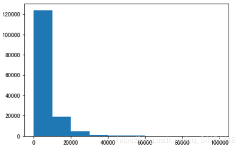
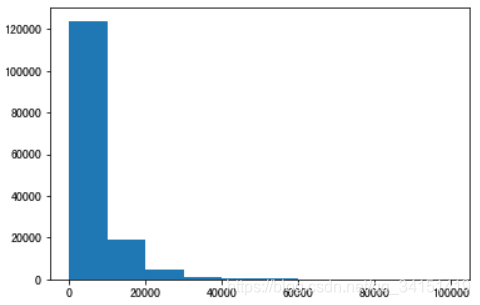
3) 统计标签的基本分布信息

print('Sta of label:')
Sta_inf(Y_data)

Sta of label:
_min 11
_max: 99999
_mean 5923.32733333
_ptp 99988
_std 7501.97346988
_var 56279605.9427

## 绘制标签的统计图，查看标签分布
plt.hist(Y_data)
plt.show()
plt.close()

4) 缺省值用-1填补

X_data = X_data.fillna(-1)
X_test = X_test.fillna(-1)

Step 4:模型训练与预测

1) 利用xgb进行五折交叉验证查看模型的参数效果

## xgb-Model
xgr = xgb.XGBRegressor(n_estimators=120, learning_rate=0.1, gamma=0, subsample=0.8,\
        colsample_bytree=0.9, max_depth=7) #,objective ='reg:squarederror'

scores_train = []
scores = []

## 5折交叉验证方式
sk=StratifiedKFold(n_splits=5,shuffle=True,random_state=0)
for train_ind,val_ind in sk.split(X_data,Y_data):
    
    train_x=X_data.iloc[train_ind].values
    train_y=Y_data.iloc[train_ind]
    val_x=X_data.iloc[val_ind].values
    val_y=Y_data.iloc[val_ind]
    
    xgr.fit(train_x,train_y)
    pred_train_xgb=xgr.predict(train_x)
    pred_xgb=xgr.predict(val_x)
    
    score_train = mean_absolute_error(train_y,pred_train_xgb)
    scores_train.append(score_train)
    score = mean_absolute_error(val_y,pred_xgb)
    scores.append(score)

print('Train mae:',np.mean(score_train))
print('Val mae',np.mean(scores))

Train mae: 628.086664863
Val mae 715.990013454

2） 定义xgb和lgb模型函数

def build_model_xgb(x_train,y_train):
    model = xgb.XGBRegressor(n_estimators=150, learning_rate=0.1, gamma=0, subsample=0.8,\
        colsample_bytree=0.9, max_depth=7) #, objective ='reg:squarederror'
    model.fit(x_train, y_train)
    return model

def build_model_lgb(x_train,y_train):
    estimator = lgb.LGBMRegressor(num_leaves=127,n_estimators = 150)
    param_grid = {
        'learning_rate': [0.01, 0.05, 0.1, 0.2],
    }
    gbm = GridSearchCV(estimator, param_grid)
    gbm.fit(x_train, y_train)
    return gbm

3）切分数据集（Train,Val）进行模型训练，评价和预测

## Split data with val
x_train,x_val,y_train,y_val = train_test_split(X_data,Y_data,test_size=0.3)

print('Train lgb...')
model_lgb = build_model_lgb(x_train,y_train)
val_lgb = model_lgb.predict(x_val)
MAE_lgb = mean_absolute_error(y_val,val_lgb)
print('MAE of val with lgb:',MAE_lgb)

print('Predict lgb...')
model_lgb_pre = build_model_lgb(X_data,Y_data)
subA_lgb = model_lgb_pre.predict(X_test)
print('Sta of Predict lgb:')
Sta_inf(subA_lgb)

Train lgb...
MAE of val with lgb: 689.084070621
Predict lgb...
Sta of Predict lgb:
_min -519.150259864
_max: 88575.1087721
_mean 5922.98242599
_ptp 89094.259032
_std 7377.29714126
_var 54424513.1104

print('Train xgb...')
model_xgb = build_model_xgb(x_train,y_train)
val_xgb = model_xgb.predict(x_val)
MAE_xgb = mean_absolute_error(y_val,val_xgb)
print('MAE of val with xgb:',MAE_xgb)

print('Predict xgb...')
model_xgb_pre = build_model_xgb(X_data,Y_data)
subA_xgb = model_xgb_pre.predict(X_test)
print('Sta of Predict xgb:')
Sta_inf(subA_xgb)

Train xgb...
MAE of val with xgb: 715.37757816
Predict xgb...
Sta of Predict xgb:
_min -165.479
_max: 90051.8
_mean 5922.9
_ptp 90217.3
_std 7361.13
_var 5.41862e+07

4）进行两模型的结果加权融合

## 这里我们采取了简单的加权融合的方式
val_Weighted = (1-MAE_lgb/(MAE_xgb+MAE_lgb))*val_lgb+(1-MAE_xgb/(MAE_xgb+MAE_lgb))*val_xgb
val_Weighted[val_Weighted<0]=10 # 由于我们发现预测的最小值有负数，而真实情况下，price为负是不存在的，由此我们进行对应的后修正
print('MAE of val with Weighted ensemble:',mean_absolute_error(y_val,val_Weighted))

MAE of val with Weighted ensemble: 687.275745703

sub_Weighted = (1-MAE_lgb/(MAE_xgb+MAE_lgb))*subA_lgb+(1-MAE_xgb/(MAE_xgb+MAE_lgb))*subA_xgb

## 查看预测值的统计进行
plt.hist(Y_data)
plt.show()
plt.close()

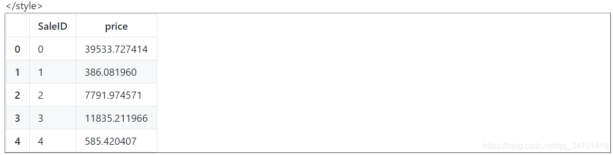
5）输出结果

sub = pd.DataFrame()
sub['SaleID'] = X_test.SaleID
sub['price'] = sub_Weighted
sub.to_csv('./sub_Weighted.csv',index=False)

sub.head()

.dataframe tbody tr th {
    vertical-align: top;
}

.dataframe thead th {
    text-align: right;
}

Baseline END.