阿里天池训练营day08：KNN分类

阿里天池训练营day08：KNN分类

1. 简介

KNN 原理和应用在day07已经叙述，这篇直接开始使用

2. 算法实践

2.1 二维数据集–knn分类

Step1: 库函数导入

import numpy as np
import matplotlib.pyplot as plt
from matplotlib.colors import ListedColormap
from sklearn.neighbors import KNeighborsClassifier
from sklearn import datasets

Step2: 数据导入

# 使用莺尾花数据集的前两维数据，便于数据可视化
iris = datasets.load_iris()
X = iris.data[:, :2]
y = iris.target

Step3: 模型训练&可视化

k_list = [1, 3, 5, 8, 10, 15]
h = .02
# 创建不同颜色的画布
cmap_light = ListedColormap(['orange', 'cyan', 'cornflowerblue'])
cmap_bold = ListedColormap(['darkorange', 'c', 'darkblue'])

plt.figure(figsize=(15,14))
# 根据不同的k值进行可视化
for ind,k in enumerate(k_list):
    clf = KNeighborsClassifier(k)
    clf.fit(X, y)
    # 画出决策边界
    x_min, x_max = X[:, 0].min() - 1, X[:, 0].max() + 1
    y_min, y_max = X[:, 1].min() - 1, X[:, 1].max() + 1
    xx, yy = np.meshgrid(np.arange(x_min, x_max, h),
                         np.arange(y_min, y_max, h))
    Z = clf.predict(np.c_[xx.ravel(), yy.ravel()])
    # 根据边界填充颜色
    Z = Z.reshape(xx.shape)

    plt.subplot(321+ind)  
    plt.pcolormesh(xx, yy, Z, cmap=cmap_light)
    # 数据点可视化到画布
    plt.scatter(X[:, 0], X[:, 1], c=y, cmap=cmap_bold,
                edgecolor='k', s=20)
    plt.xlim(xx.min(), xx.max())
    plt.ylim(yy.min(), yy.max())
    plt.title("3-Class classification (k = %i)"% k)

plt.show()

Step4: 原理简析

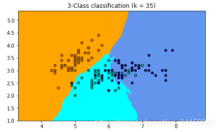
如果选择较小的K值，就相当于用较小的领域中的训练实例进行预测，例如当k=1的时候，在分界点位置的数据很容易受到局部的影响，图中蓝色的部分中还有部分绿色块，主要是数据太局部敏感。当k=15的时候，不同的数据基本根据颜色分开，当时进行预测的时候，会直接落到对应的区域，模型相对更加鲁棒。

增大k时，先看数据集大小

y = iris.target
print(y.shape)
# (150,)

让k=100和k=120时，分类的结果与前面的有很大的区别，主要是下和右两类的界限在明显的改变，黄色的由于数据很聚集，并没有太影响，就这批数据而言，整体上还是比较明显的有聚类，因此在增大k时，对聚类中心的影响没有想象那么明显。

2.2 莺尾花数据集–kNN分类

Step1: 库函数导入

# 从sklearn.datasets 导入 iris数据加载器。
from sklearn.datasets import load_iris
# 从sklearn.model_selection  里选择导入train_test_split用于数据分割。
from sklearn.model_selection  import train_test_split
# 从sklearn.preprocessing里选择导入数据标准化模块。
from sklearn.preprocessing import StandardScaler
# 从sklearn.neighbors里选择导入KNeighborsClassifier，即K近邻分类器。
from sklearn.neighbors import KNeighborsClassifier

Step2: 数据导入&分析

# 使用加载器读取数据并且存入变量iris。
iris = load_iris()
# 查验数据规模。
iris.data.shape
##(150, 4)
# 查看数据说明
print(iris.DESCR)
'''
Iris plants dataset
--------------------

**Data Set Characteristics:**

    :Number of Instances: 150 (50 in each of three classes)
    :Number of Attributes: 4 numeric, predictive attributes and the class
    :Attribute Information:
        - sepal length in cm
        - sepal width in cm
        - petal length in cm
        - petal width in cm
        - class:
                - Iris-Setosa
                - Iris-Versicolour
                - Iris-Virginica
                
    :Summary Statistics:

    ============== ==== ==== ======= ===== ====================
                    Min  Max   Mean    SD   Class Correlation
    ============== ==== ==== ======= ===== ====================
    sepal length:   4.3  7.9   5.84   0.83    0.7826
    sepal width:    2.0  4.4   3.05   0.43   -0.4194
    petal length:   1.0  6.9   3.76   1.76    0.9490  (high!)
    petal width:    0.1  2.5   1.20   0.76    0.9565  (high!)
    ============== ==== ==== ======= ===== ====================

    :Missing Attribute Values: None
    :Class Distribution: 33.3% for each of 3 classes.
    :Creator: R.A. Fisher
    :Donor: Michael Marshall (MARSHALL%PLU@io.arc.nasa.gov)
    :Date: July, 1988

The famous Iris database, first used by Sir R.A. Fisher. The dataset is taken
from Fisher's paper. Note that it's the same as in R, but not as in the UCI
Machine Learning Repository, which has two wrong data points.
'''
# 使用train_test_split，利用随机种子random_state采样25%的数据作为测试集。
X_train, X_test, y_train, y_test = train_test_split(iris.data, iris.target, test_size=0.25, random_state=33)

Step3: 模型训练

# 对训练和测试的特征数据进行标准化。
ss = StandardScaler()
X_train = ss.fit_transform(X_train)
X_test = ss.transform(X_test)
 
# 使用K近邻分类器对测试数据进行类别预测，预测结果储存在变量y_predict中。
knc = KNeighborsClassifier()
knc.fit(X_train, y_train)
y_predict = knc.predict(X_test)
 

Step4: 模型预测

# 使用模型自带的评估函数进行准确性测评。
print ('The accuracy of K-Nearest Neighbor Classifier is', knc.score(X_test, y_test) )
## The accuracy of K-Nearest Neighbor Classifier is 0.8947368421052632
# 依然使用sklearn.metrics里面的classification_report模块对预测结果做更加详细的分析。
from sklearn.metrics import classification_report
print (classification_report(y_test, y_predict, target_names=iris.target_names))
'''
                precision    recall  f1-score   support

      setosa       1.00      1.00      1.00         8
  versicolor       0.73      1.00      0.85        11
   virginica       1.00      0.79      0.88        19

    accuracy                           0.89        38
   macro avg       0.91      0.93      0.91        38
weighted avg       0.92      0.89      0.90        38
'''

3. 总结

对于使用机器学习库做分类或者回归任务时，模型本身已经不是最重要的了，因为模型基本上是固定的，大部分的内容是读取数据，对数据清晰、分类、分隔，按照模型的需要做相应的处理送入模型。