机器学习2梯度下降求解逻辑回归

案例：

案例：
建立一个逻辑回归模型预测一个学生是否可以被录取。
根据两次考试的结果来决定每个申请人的录取机会，有以前申请人的历史数据，用它作为逻辑回归的训练集，建立一
个分类模型，根据考试成绩估计入学概率。

#准备工作，导入包

import numpy as np
import pandas as pd
import matplotlib.pyplot as plt   

#读取文件

import os
path = 'data' +os.sep+'LogReg_data.txt'
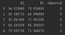
pdData = pd.read_csv(path,header=None,names=['E1','E2','Admitted'])
pdData.head()
pdData.shape

### os.sep 根据你所处的平台,自动地采用相应的分割符号
### head() 默认输出五行

#数据可视化展示

positive = pdData[pdData['Admitted']==1]
negative = pdData[pdData['Admitted']==0]
fig,ax = plt.subplots(figsize=(10,5))
ax.scatter( positive['E1'],positive['E2'],c='r',marker='o', label='Admitted' )
ax.scatter( negative['E1'],positive['E2'],c='b',marker='x', label='Not Admitted')
ax.set_xlabel('E1 sources')
ax.set_ylabel('E2 sources')
plt.show()

The logistic regression
目标：建立分类器（求解出三个参数012）
设定阈值，根据阈值判断录取结果

要完成的模块
sigmod:映射到概率的函数
model:返回预测结果值
cost:根据参数计算损失
gradient:计算每个参数的梯度方向
descent:进行参数更新
accuracy:计算精度

sigmod函数:

def sigmoid(Z):
    return 1/(1 + np.exp(-z))

模型函数：

def model(X,theta):
    return sigmoid(np.dot(X,theta.T))

pdData.insert(0,'Ones',1)               #首列插入全是1的值
orig_data = pdData.as_matrix()     #数据格式转化为矩阵
cols = orig_data.shape[1]
X=orig_data[:,0:cols-1]                  #提取特征
y =orig_data[:,cols-1:cols]              #提取标签
theta = np.zeros([1,3])                  #初始化三个参数

#计算损失

def cost(X,y,theta):
    left = np.multiply(-y,np.log(model(X,theta)))
    right = np.multiply(1-y,np.log(1-model(X,theta)))
    return np.sum(left - right)/(len(X))          #根据似然函数的目标函数列式

#计算梯度

def gradient(X,y,theta):
    grad = np.zeros(theta.shape)                 #初始化梯度参数
    error = (model(X,theta)-y).ravel()
    for j in range(len( theta.ravel()) ):            #遍历对每一个参数求偏导
        term = np.multiply(error,X[:,j])
        grad[0,j] = np.sum(term)/len(X）
    return grad

STOP_ITER = 0                       #根据迭代次数终止
STOP_COST = 1                       #根据损失值终止
STOP_GRAD = 2                       #根据梯度终止
def stopCriterion(type,value,threshold):
    #设定三种不同的策略
    if type == STOP_ITER:       return value>threshold                      #threshold 指定阈值
    elif type == STOP_COST:   return abs(value[-1]-value[-2])<threshold
    elif type == STOP_GRAD:   return np.linalg.norm(value)<threshold

import numpy.random
#洗牌
def shuffleData(data):
    np.random.shuffle(data)
    cols = data.shape[1]
    X = data[:, 0:cols-1]
    y = data[:, cols-1: ]
    return X,y

import time
def descent(data, theta, batchSize,stopType,thresh,alpha):
    #梯度下降求解
    init_time = time.time()
    i =0  #迭代次数
    k=0 # batch
    X,y = shuffleData(data)
    grad = np.zeros(theta.shape) #计算的梯度
    costs = [cost(X,y,theta)]
    while True:
        grad = gradient(X[k:k+batchSize],y[k:k+batchSize],theta)
        k += batchSize  #取batch数量个数据
        if k>= n:
            k=0
            X,y = shuffleData(data)       #重新洗牌
        theta = theta - alpha*grad       #参数更新
        costs.append(cost(X,y,theta))   #计算新的损失
        i+=1    
        if stopType == STOP_ITER:    value = i
        elif stopType == STOP_COST:  value = costs
        elif stopType == STOP_GRAD: value = grad
        if stopCriterion(stopType,value,thresh):break
    return theta,i-1,costs,grad,time.time() - init_time

def runExpe(data,theta,batchSize,stopSize,thresh,alpha):
    theta,iter,costs,grad,dur = descent(data,theda,batchSize,stopType,thresh,alpha)
    name = "Original" if (data[:,1]>2).sum()>1 else "Scaled"
    name +="data - learning rate:{} -".format(alpha)
    if batchSize ==n:strDescType = "Gradient"
    elif batchSize == 1:strDescType = "Stochastic"
    else:strDescType = "Mini-batch({ })".format(batchSize)
    name += strDescType+"descent-Stop:"

    if stopType == STOP_ITER:strStop="{} iterations".format(thresh)
    elif stopType ==STOP_COST:strStop="costs change <{}".format(thresh)
    else :strStop ="gradient norm<{}".format(thresh)
    name +=strStop
    print("")
    fig,ax = plt.subplots(figsize=(12,4))
    ax.plot(np.arange(len(costs)),costs,'r')
    ax.set_xlabel('Iterations')
    ax.set_ylabel('Cost')
    ax.set_title(name.upper()+' -Error vs.Iteration')
    return theta 

#精度：
def predict(X,theta):
    return [1 if x >=0.5 else 0 for x in model(X,theta)]

scaled_X = scaled_data[:, :3]
y = scaled_data[:,3]
predictions = predict(scaled_X,theta)
correct = [1 if ((a == 1 and b==1) or (a==0 and b==0)) else 0 for(a,b) in zip(predictions,y)]
accuracy = (sum(map(int,correct))%len(correct) )
print('accuracy={0}%'.format(accuracy))