不使用深度模型框架，只利用Tensor和autograd来实现一个线性回归的训练

步骤：
1. 读取输入数据 
2. 使用正态分布生成读取直线的散点
3. 定义网络结构 定义loss等参数
4. 使用Tensor和autograd迭代更新 进行回归


代码如下：

import torch
from matplotlib import pyplot as plt
import numpy as np
import random

# 得到输入、标签features, labels
num_inputs = 2

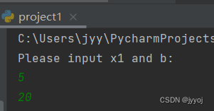
print('Please input x1 and b:')
x1 = int(input())
b = int(input())

num_example = 1000
true_w = [x1, -1]

# true_w 类型要求是 [x, -1] 其中x可以是任何数

true_b = b
features = torch.randn(num_example, num_inputs, dtype=torch.float32)
labels = true_w[0] * features[:, 0] + true_w[1] * features[:, 1] + true_b
labels += torch.tensor(np.random.normal(0, 0.01, size=labels.size()), dtype=torch.float32)

plt.scatter(features[:, 0].numpy(), labels.numpy(), 1)
# plt.show()


# 二、准备数据生成器，每次生成我们所需要的batch_size大小的数据和标签
def data_iter(batch_size, features, labels):
    num_examples = len(features)
    indices = list(range(num_examples)) # 列表 [0，…… ,num_examples-1]
    random.shuffle(indices)
    for i in range(0, num_examples, batch_size):# start, stop, step
        j = torch.LongTensor(indices[i:min(i + batch_size, num_examples)]) # 最后一次可能不足一个batch
        yield features.index_select(0, j), labels.index_select(0, j) # dim , index


batch_size = 10

# 查看生成的数据
# for X, y in data_iter(batch_size, features, labels):
#     print(X, y)
#break

# 三、初始化参数
w = torch.tensor(np.random.normal(0, 0.01, (num_inputs, 1)), dtype=torch.float32, requires_grad=True)
b = torch.zeros(1, dtype=torch.float32, requires_grad=True)

# print(w)
# print(b)

# 四、定义网络结构，
def linreg(X, w, b):
    return torch.mm(X, w) + b
# 定义损失
def squared_loss(y_hat, y):
    return (y_hat - y.view(y_hat.size())) ** 2 / 2

# 定义更新参数方式
def sgd(params, lr, batch_size):
    for param in params:
        param.data -= lr * param.grad / batch_size
# 改变data，改变参数值

lr = 0.02
num_epochs = 50
net = linreg
loss = squared_loss

# 开始迭代
for epoch in range(num_epochs):
    for X, y in data_iter(batch_size, features, labels):
        l = loss(net(X, w, b), y).sum()
        # l = l.sum()
        l.backward()
        sgd([w, b], lr, batch_size)
        w.grad.data.zero_()
        b.grad.data.zero_()
    train_l = loss(net(features, w, b), labels)
    print('epoch %d, loss %f' % (epoch+1, train_l.mean().item())) # item是得到一个元素张量里面的元素值

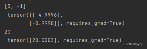
print(true_w, '\n', w)
print(true_b, '\n', b)

x1 = -5
x2 = 5
y1 = (true_w[0] * x1 ) / (-true_w[1]) + true_b
y2 = (true_w[0] * x2 ) / (-true_w[1]) + true_b

plt.plot([x1, x2], [y1, y2], 'b-', label='Line')
plt.show()

输入：

 输出：