


流程
在
N
w
a
y
−
K
s
h
o
t
N way - K shot
Nway−Kshot的
e
p
i
s
o
d
e
episode
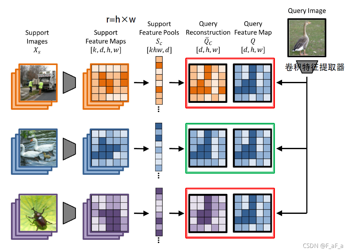
episode下(图中N=K=3,有3个类,每类有3张图片),
X
s
X_s
Xs表示支持图片的集合.当有单张查询图片
x
q
x_q
xq的时候,我们希望能预测它的标签
y
q
y_q
yq.
灰色的梯形代表卷积特征提取器, x q x_q xq经过它产生的一个大小为 r × d r×d r×d大小的特征图输出(记作 Q Q Q),其中 r = h × w r = h×w r=h×w代表空间大小, d d d是通道数.
对于 C C C个类别,我们把每个类的 k k k个图片通过卷积特征提取器转换成特征图 S c S_c Sc,大小为 k r × d kr×d kr×d(因为有k个图片的特征,每个特征图大小为 r × d r×d r×d)
我们想找到矩阵
W
W
W,这样把
Q
Q
Q表示为矩阵乘法
W
×
S
c
≈
Q
W ×S_c ≈ Q
W×Sc≈Q,求出最优
W
ˉ
\bar{W}
Wˉ等于求解线性最小二乘问题
W
ˉ
=
arg
min
W
∥
Q
−
W
S
c
∥
2
+
λ
∥
W
∥
2
\bar{W}=\underset{W}{\arg \min }\left\|Q-W S_{c}\right\|^{2}+\lambda\|W\|^{2}
Wˉ=Wargmin∥Q−WSc∥2+λ∥W∥2
通过岭回归公式可以得出最优的
W
ˉ
\bar{W}
Wˉ和
Q
c
ˉ
\bar{Q_c}
Qcˉ
W
ˉ
=
Q
S
c
T
(
S
c
S
c
T
+
λ
I
)
−
1
Q
ˉ
c
=
W
ˉ
S
c
\begin{aligned} &\bar{W}=Q S_{c}^{T}\left(S_{c} S_{c}^{T}+\lambda I\right)^{-1} \\ &\bar{Q}_{c}=\bar{W} S_{c} \end{aligned}
Wˉ=QScT(ScScT+λI)−1Qˉc=WˉSc
对于给定的类c,把
Q
Q
Q和
Q
c
ˉ
\bar{Q_c}
Qcˉ之间距离定义为欧氏距离,然后用
1
r
\frac{1}{r}
r1进行放缩。在所有C个类上,距离乘上
−
γ
-\gamma
−γ做softmax,公式如下:
⟨
Q
,
Q
ˉ
c
⟩
=
1
r
∥
Q
−
Q
ˉ
c
∥
2
P
(
y
q
=
c
∣
x
q
)
=
e
(
−
γ
⟨
Q
,
Q
ˉ
c
⟩
)
∑
c
′
∈
C
e
(
−
γ
⟨
Q
,
Q
ˉ
c
′
⟩
)
\begin{aligned} \left\langle Q, \bar{Q}_{c}\right\rangle &=\frac{1}{r}\left\|Q-\bar{Q}_{c}\right\|^{2} \\ P\left(y_{q}=c \mid x_{q}\right) &=\frac{e^{\left(-\gamma\left\langle Q, \bar{Q}_{c}\right\rangle\right)}}{\sum_{c^{\prime} \in C} e^{\left(-\gamma\left\langle Q, \bar{Q}_{c^{\prime}}\right\rangle\right)}} \end{aligned}
⟨Q,Qˉc⟩P(yq=c∣xq)=r1∥∥Q−Qˉc∥∥2=∑c′∈Ce(−γ⟨Q,Qˉc′⟩)e(−γ⟨Q,Qˉc⟩)
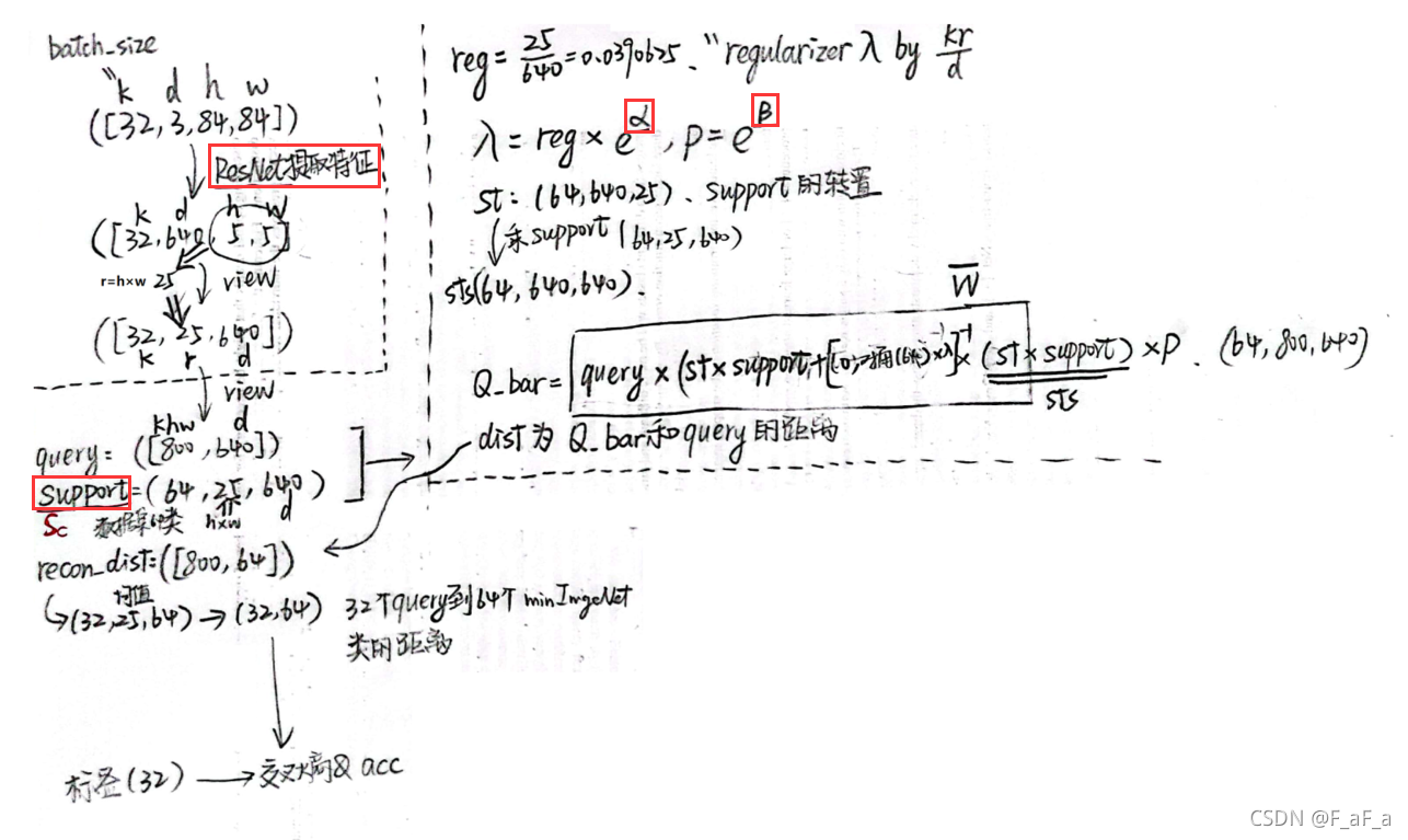
求解公式 W ˉ = arg min W ∥ Q − W S c ∥ 2 + λ ∥ W ∥ 2 \bar{W}=\underset{W}{\arg \min }\left\|Q-W S_{c}\right\|^{2}+\lambda\|W\|^{2} Wˉ=Wargmin∥Q−WSc∥2+λ∥W∥2的难度是变化的:
- 如果kr > d, 解出来是比较容易的
- 如果kr < d, 解出来很麻烦,这个时候就需要改进公式了
为了保证训练的稳定性,于是决定用
1
k
r
\frac{1}{kr}
kr1改进
λ
\lambda
λ,这有一个额外的好处,使我们的模型在某种程度上健壮.
另外
λ
\lambda
λ应该是学习来的参数。改变
λ
\lambda
λ有多样的效果:大的
λ
\lambda
λ避免过分依赖
W
W
W的权重,但是也降低了重建的效果、增加了重建的error、限制了可区分的能力。
We therefore disentangle the degree of regularization from the magnitude of Qc by introducing a learned recalibration term ρ:
因此,我们通过引入学习的重新校准项,从 Qc 的大小中解开正则化程度 ρ
这句没看懂/(ㄒoㄒ)/~~
得到公式 Q ˉ c = ρ W ˉ S c \bar{Q}_{c}=\rho \bar{W} S_{c} Qˉc=ρWˉSc
λ \lambda λ和 ρ \rho ρ 被参数化为 e α e^α eα 和 e β e^β eβ 以确保非负性,并且初始化为零。
因此,总而言之,我们的最终预测由下式给出:
λ
=
k
r
d
e
α
ρ
=
e
β
Q
ˉ
c
=
ρ
W
ˉ
S
c
=
ρ
Q
S
c
T
(
S
c
S
c
T
+
λ
I
)
−
1
S
c
P
(
y
q
=
c
∣
x
q
)
=
e
(
−
γ
⟨
Q
,
Q
ˉ
c
⟩
)
∑
c
′
∈
C
e
(
−
γ
⟨
Q
,
Q
ˉ
c
′
⟩
)
\begin{gathered} \lambda=\frac{k r}{d} e^{\alpha} \quad \rho=e^{\beta} \\ \bar{Q}_{c}=\rho \bar{W} S_{c}=\rho Q S_{c}^{T}\left(S_{c} S_{c}^{T}+\lambda I\right)^{-1} S_{c} \\ P\left(y_{q}=c \mid x_{q}\right)=\frac{e^{\left(-\gamma\left\langle Q, \bar{Q}_{c}\right\rangle\right)}}{\sum_{c^{\prime} \in C} e^{\left(-\gamma\left\langle Q, \bar{Q}_{c^{\prime}}\right\rangle\right)}} \end{gathered}
λ=dkreαρ=eβQˉc=ρWˉSc=ρQScT(ScScT+λI)−1ScP(yq=c∣xq)=∑c′∈Ce(−γ⟨Q,Qˉc′⟩)e(−γ⟨Q,Qˉc⟩)
该算法只引入了3个可以学习的参数:
α
,
β
,
γ
\alpha,\beta,\gamma
α,β,γ
公式 Q ˉ c = ρ W ˉ S c = ρ Q S c T ( S c S c T + λ I ) − 1 S c \bar{Q}_{c}=\rho \bar{W} S_{c}=\rho Q S_{c}^{T}\left(S_{c} S_{c}^{T}+\lambda I\right)^{-1} S_{c} Qˉc=ρWˉSc=ρQScT(ScScT+λI)−1Sc中
- 在 k r < d kr \lt d kr<d的时候容易计算。因为最麻烦的一步是求 k r × k r kr×kr kr×kr矩阵的逆,和d没有关系;从左到右计算矩阵乘积也避免了在内存中存储一个可能很大的d×d矩阵
- 但是在特征图很大或者
d
<
k
r
d \lt kr
d<kr的时候,这个公式将会很麻烦。此时可以将公式变为下面的公式,最昂贵的步骤是
d
×
d
d × d
d×d矩阵的求逆,从右到左计算乘积避免了内存中保存大型
k
r
×
k
r
kr×kr
kr×kr或
b
r
×
k
r
br×kr
br×kr矩阵。
Q ˉ c = ρ W ˉ S c = ρ Q ( S c T S c + λ I ) − 1 S c T S c \bar{Q}_{c}=\rho \bar{W} S_{c}=\rho Q\left(S_{c}^{T} S_{c}+\lambda I\right)^{-1} S_{c}^{T} S_{c} Qˉc=ρWˉSc=ρQ(ScTSc+λI)−1ScTSc
代码
其中红色方框就是模型要学习的参数
一些疑问
作者邮件回复了我的问题
- 代码没找到
Auxiliary Loss的实现
作者回复我
The code for the auxiliary loss can be found in trainers/frn_train.py, lines 9-26.
- 代码和代码获取
S
c
S_c
Sc的方式不一样
论文中的 S c S_c Sc明明是特征图变幻得来,代码中却变成了learnable parameter,奇怪。
The paper and code get Sc in different ways.
In the code , Sc is a learnable parameter in the FRN model.
In the figure2 of paper, the support Images(N way - K shot) gets the feature map [k,d,h,w] through convolutional feature extractor, and reshape the feature map into [khw,d].
作者回复我
The source of S_c depends on whether you are training or pretraining the FRN model.
When pretraining, S_c is indeed a learned layer at the top of the network. This is only used for mini-ImageNet experiments in the pretraining stage.
Otherwise, S_c corresponds to the reshaped pool of support features (using get_neg_l2_distance() instead of forward_pretrain() in models/FRN.py).
- 代码没找到
Reconstruction Visualization的实现
作者回复我
We hadn’t planned on publishing the visualization code but I’m happy to share what we do have.
Unfortunately we had to do a fair amount of adaptation from our working code to the github version, so what I’m sending is mildly sanitized working code and not nicely integrated.
It’s a jupyter notebook - you will have to set some values and imports manually, but after that it should run straightforwardly (load a feature extractor, train the image decoder, evaluate reconstruction error, generate figures).


 被折叠的 条评论
为什么被折叠?
被折叠的 条评论
为什么被折叠?
 到【灌水乐园】发言


