[学习笔记]逻辑回归笔记（二）

最新推荐文章于 2022-11-22 23:00:07 发布

student_mei

最新推荐文章于 2022-11-22 23:00:07 发布

阅读量1k

点赞数 1

分类专栏： Python个人学习笔记

本文链接：https://blog.csdn.net/qq_38308533/article/details/80294645

版权

Python个人学习笔记专栏收录该内容

7 篇文章 1 订阅

订阅专栏

吴恩达机器学习课后作业总结
代码参考黄海广
自己学习记录所用
数据集来自课后作业exercise2

一、线性可分的逻辑回归分类问题

初始化部分

import numpy as np
import pandas as pd
from pandas import Series,DataFrame
import matplotlib.pyplot as plt
import matplotlib
data = pd.read_csv('ex2data1.txt',names=['Exam1_Score','Exam2_Score','Admitte_Label'])
Label_classify = data.Admitte_Label.values == True  #得到一个bool型数组(array)
Score=data[['Exam1_Score','Exam2_Score']]  #要取出DataFrame的两列及以上的数据时，传入的是一个list，[...]。此时得到的输出仍是一个DataFrame
                                           #若取出一个数据，如data[['Exam1_Score']]时，得到的仍是一个DataFrame
Admitted,Not_Admitted = Score[Label_classify],Score[~Label_classify]#对DataFrame传入一个bool型数组，会过滤掉行（即按行进行提取数据）
plt.figure(1,figsize=(12,8))
plt.scatter(Admitted['Exam1_Score'],Admitted['Exam2_Score'],c='black',marker='+',s=100,linewidths=3)
plt.scatter(Not_Admitted['Exam1_Score'],Not_Admitted['Exam2_Score'],c='yellow',marker='o',s=100,linewidths=3)

结果如下：
这里写图片描述
从直观上很容易看到，这个是一个线性可分的二分类问题，即只要找出线性边界就能够对数据进行切分
- 采用逻辑回归，因此首先写出sigmoid函数：

def sigmoid(z):       #s函数
    return 1/(1+np.exp(-z))

对于逻辑回归，我们知道其代价函数为：
$J(\theta)=\frac{1}{m}\sum_{i=1}^mCost(h_\theta(x^{(i)},y^{(i)}))$ ，其中

$Cost(h_\theta(x),y)=\begin{cases} -log(h_\theta(x)),if \ \ \ y=1\\ -log(1-h_\theta(x)),if \ \ \ y=0\\ \end{cases}$
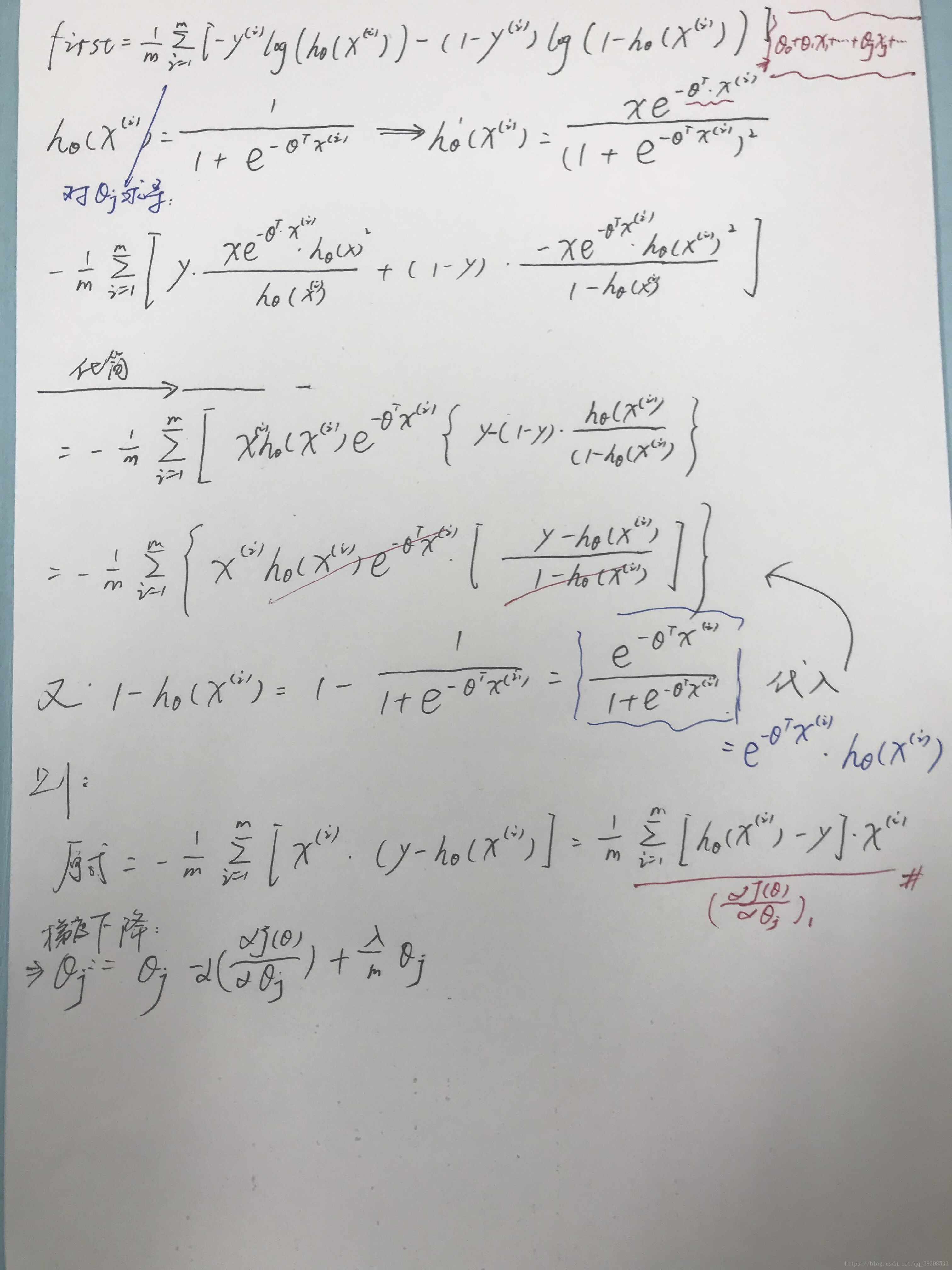
据此，写出代价函数和进行一次梯度下降后函数表达式分别如下：
- 代价函数：

def cost(theta,X,y):#代价函数，传入的theta待迭代更新，X为数据集，y为数据集对应标签
    X = np.matrix(X)
    y = np.matrix(y)
    h_x = sigmoid(theta*X.T)
    L = np.multiply(y.T,np.log(h_x))+np.multiply((1-y).T,np.log(1-h_x))  #np.log(X)是分别对X中每一个元素求log,1-y会出现广播的情况
    return (-np.sum(L))/(len(X))

进行一次梯度下降后的表达式（即对于某一时刻的 $\theta$ 得到的导数–> $\frac{1}{m}\sum_{i=1}^{m}(h_\theta(x^{(i)}-y^{(i)})x_j^{(i)}$ )：

def costgradient(theta,X,y):
    theta = np.matrix(theta)
    X = np.matrix(X)
    y = np.matrix(y)
    gradient_value= np.sum(np.multiply((sigmoid(X*theta.T)-y),X),axis=0)/(len(X))
#     theta = theta - alpha*gradient_value[i,:]
    return gradient_value

用SciPy’s truncated newton（TNC）实现寻找最优参数

import scipy.optimize as opt
result = opt.fmin_tnc(func=cost, x0=theta, fprime=costgradient, args=(X, y)) ##（暂时不太明白）
result #result中，第一个数是更新后的theta
##result：
    (array([-25.16131861,   0.20623159,   0.20147149]), 36, 0)

进行预测——由于是二分类问题，因此只有两个标签（0、1），因此，只需根据sigmoid函数的状态直接对数据进行分析即可：

def predict(theta,X):
    X = np.matrix(X)
    theta = np.matrix(theta)
    z = X*theta.T
    h_x = sigmoid(z)
    return [1 if h_x[i] >= 0.5 else 0 for i in range(len(np.array(h_x)))]

测试：

predict_score = np.array(predict(result[0],X))
true_score = y.values.ravel()
predict_out = np.array([1 if ((i==1 and j ==1) or (i==0 and j ==0)) else 0 for i,j in zip(predict_score,true_score)])
ratio = sum(predict_out == 1)/len(predict_out)
print("accuracy is {0}%".format(ratio*100))

找出决策边界
$X \times \theta = 0$ (this is the line)
因此对于只有两个特征的这一情况，有：
$θ 0 + θ 1 x 1 + θ 2 x 2 = 0$ $\theta_0+\theta_1x_1+\theta_2x_2=0$
将 $x2$ 看为y，则：
$y =-\frac{\theta_0}{\theta_2}-\frac{\theta_1}{\theta_2}x_1$
据此，可得到：

theta_opt = result[0] #由scipy.optimize函数得到的经过梯度下降后更新的theta数据
##result[0] ----->
    array([-25.16131861,   0.20623159,   0.20147149])
theta_opt.tolist()/result[0][0]
###----->
    array([ 1.        , -0.00819637, -0.00800719])
coef = (-result[0]/result[0][-1]).tolist()
print(coef)
    ###[124.88774020181867, -1.02362667995475, -1.0]
x = np.arange(100, step=0.1)
f_x = coef[0] + coef[1]*x   

##可视化
plt.figure(3,figsize=(12,8))
plt.scatter(Admitted['Exam1_Score'],Admitted['Exam2_Score'],c='black',marker='+',s=100,label='Admitted',linewidths=3)
plt.scatter(Not_Admitted['Exam1_Score'],Not_Admitted['Exam2_Score'],c='yellow',marker='o',s=100,linewidths=3,label='Rejected')
plt.plot(x,f_x)
plt.xlim(30,100)
plt.ylim(30,100)
plt.title('Decision Boundary')
plt.xlabel('Exam1_Score')
plt.ylabel('Exam2_Score')
plt.legend(['Boundary','Admitted','Rejected'])

这里写图片描述

二、正则化逻辑回归

data2=pd.read_csv('ex2data2.txt',header=None, names=['Test 1', 'Test 2', 'Accepted'])
plt.figure(4,figsize=(12,8))
plt.scatter(positive_test.iloc[:,0],positive_test.iloc[:,1],c='black',marker='+',s=100,linewidths=3,label='y=1')
plt.scatter(negtive_test.iloc[:,0],negtive_test.iloc[:,1],c='yellow',marker='o',s=100,linewidths=3,label='y=1')
plt.xlim(-1,1.5)
plt.ylim(-0.8,1.2)
plt.xlabel('Microchip Test 1')
plt.ylabel('Microchip Test 2')
plt.title('lambda = 1')
plt.legend(['y=1','y=0'])

这里写图片描述

feature mapping（特征映射）

polynomial expansion

for i in 0..i
for p in 0..i:
output x^(i-p) * y^p
特征映射
据此，有：

def feature_mapping(x, y, power, as_ndarray=False):
#     """return mapped features as ndarray or dataframe"""
    # data = {}
    # # inclusive
    # for i in np.arange(power + 1):
    #     for p in np.arange(i + 1):
    #         data["f{}{}".format(i - p, p)] = np.power(x, i - p) * np.power(y, p)

    data = {"f{}{}".format(i - p, p): np.power(x, i - p) * np.power(y, p)
                for i in np.arange(power + 1)
                for p in np.arange(i + 1)
            }

    if as_ndarray:
        return pd.DataFrame(data).as_matrix()
    else:
        return pd.DataFrame(data)

regularized cost（正则化代价函数）

J (θ) = 1 m \sum i = 1 m [- y (i) log (h θ (x (i))) - (1 - y (i)) log (1 - h θ (x (i)))] + λ 2 m \sum j = 1 n θ 2 j

$J\left( \theta \right)=\frac{1}{m}\sum\limits_{i=1}^{m}{[-{{y}^{(i)}}\log \left( {{h}_{\theta }}\left( {{x}^{(i)}} \right) \right)-\left( 1-{{y}^{(i)}} \right)\log \left( 1-{{h}_{\theta }}\left( {{x}^{(i)}} \right) \right)]}+\frac{\lambda }{2m}\sum\limits_{j=1}^{n}{\theta _{j}^{2}}$

def RegularCost(theta,X,y,lamta):
    X = np.matrix(X)
    y = np.matrix(y)
    theta = np.matrix(theta)
    return cost(theta,X,y)+lamta*np.sum(np.power(theta[:,1:theta.shape[1]],2))/(2*len(X))

regularized gradient(正则化梯度)

\partial J ( θ ) \partial θ j = (1 m \sum i = 1 m (h θ (x (i)) - y (i))) x (i) + λ m θ j for j \geq 1

$\frac{\partial J\left( \theta \right)}{\partial {{\theta }_{j}}}=\left( \frac{1}{m}\sum\limits_{i=1}^{m}{\left( {{h}_{\theta }}\left( {{x}^{\left( i \right)}} \right)-{{y}^{\left( i \right)}} \right)} \right)x^{(i)}+\frac{\lambda }{m}{{\theta }_{j}}\text{ }\text{ for j}\ge \text{1}$

def regularized_gradient(theta, X, y, l=1):
#     '''still, leave theta_0 alone'''
    theta_j1_to_n = theta[1:]
    regularized_theta = (l / len(X)) * theta_j1_to_n

    # by doing this, no offset is on theta_0
        regularized_term = np.concatenate([np.array([0]), regularized_theta])

    return gradient(theta, X, y) + regularized_term

其余步骤类似上文

三、多类分类问题

吴恩达机器学习exercise3
初始化工作，引入scipy包来打开.mat文件

import numpy as np
import pandas as pd
import matplotlib.pyplot as plt
from scipy.io import loadmat
data = loadmat('ex3data1.mat')

注意：

如果用的引用是import scipy而不是from scipy.io import loadmat，那么，调用时，使用scipy.io.loadmat时会报错（why？）
def lrCostFunction(theta,X,y,learningRate):
基本初始化操作：
（1）建立包含正则化的代价函数lrCostFunction(theta,X,y,learningRate)，方法类似上面
（2）建立包含正则化的梯度计算函数RegularCostGradient(theta,X,y,lamta)
（3）构建One-Vs-All多分类器
对于分类器：
现在我们已经定义了代价函数和梯度函数，现在是构建分类器的时候了。对于这个任务，我们有10个可能的类，并且由于逻辑回归只能一次在2个类之间进行分类，我们需要多类分类的策略。在本练习中，我们的任务是实现一对一全分类方法，其中具有k个不同类的标签就有k个分类器，每个分类器在“类别 i”和“不是 i”之间决定。我们将把分类器训练包含在一个函数中，该函数计算10个分类器中的每个分类器的最终权重，并将权重返回为k X（n + 1）数组，其中n是参数数量。
- 函数应该返回一个 $\Theta\in R^{K\times(N+1)}$ 所有的分类参数，K为所有可能的类别，N为样本的特征数
- $\Theta$ 对应于一个类的学习逻辑回归参数。
- 注意：该函数的y参数是从1到10的向量标签，我们将数字0映射到10

from scipy.optimize import minimize
def oneVsAll(X,y,num_labels,learning_rate):         #输入的X，y是未经过插入Ones的原始数据和对应数据集的标签
    rows = X.shape[0]
    params = X.shape[1]

    # k X (n + 1) array for the parameters of each of the k classifiers
    all_theta = np.zeros((num_labels, params + 1))#生成(num_labels)*(params + 1)的初始l零矩阵

    # insert a column of ones at the beginning for the intercept term
    X = np.insert(X, 0, values=np.ones(rows), axis=1)#对X插入Ones数据

    # labels are 1-indexed instead of 0-indexed
    for i in range(1, num_labels + 1):#一个i代表一种分类器的标号（i=1表示是第一种分类器）
        theta = np.zeros(params + 1)
        y_i = np.array([1 if label == i else 0 for label in y])#每遍历到一个分类器，就找出这个分类器在原始数据标签中的位置
        y_i = np.reshape(y_i, (rows, 1))

        # minimize the objective function
        fmin = minimize(fun=lrCostFunction, x0=theta, args=(X, y_i, learning_rate), method='TNC', jac=RegularCostGradient)#对当前的分类器找出最小的theta
        all_theta[i-1,:] = fmin.x#找出一组theta则记录一组

    return all_theta

我们现在准备好最后一步 - 使用训练完毕的分类器预测每个图像的标签。对于这一步，我们将计算每个类的类概率，对于每个训练样本（使用当然的向量化代码），并将输出类标签为具有最高概率的类。

def predict(X,all_theta):
    X = np.matrix(X)
    all_theta = np.matrix(all_theta)
    h = sigmoid(X*all_theta.T)
    h_max = np.argmax(h,axis=1)
    h_max = h_max+1
    return h_max
def predict_all(X, all_theta):#对于已经找到的theta，对应的是使得代价函数cost最小时候的最优权重theta数值；因此将X*theta.T通过sigmoid函数后，
                              #sigmoid输出的数值y对于y轴上的10个标签，每个标签都会得到一个数据，判断最大值的标签对应的位置，即表示此时predict
                              #所识别的数字是多少
    rows = X.shape[0]
    params = X.shape[1]
    num_labels = all_theta.shape[0]

    # same as before, insert ones to match the shape
    X = np.insert(X, 0, values=np.ones(rows), axis=1)

    # convert to matrices
    X = np.matrix(X)
    all_theta = np.matrix(all_theta)

    # compute the class probability for each class on each training instance
    h = sigmoid(X * all_theta.T)

    # create array of the index with the maximum probability
    h_argmax = np.argmax(h, axis=1)#1代表行--即找出每一行最大值对应的索引的位置，表示找出K个预测值中，可能性最高的一个预测值，当作此时的模型预测输出值。h_argmax在这里是(5000,1)的矩阵

    # because our array was zero-indexed we need to add one for the true label prediction
    h_argmax = h_argmax + 1

    return h_argmax

测试输出：

y_pred = predict(X, all_theta)
correct = [1 if a == b else 0 for (a, b) in zip(y_pred, data['y'])]
accuracy = (sum(map(int, correct)) / float(len(correct)))
print ('accuracy = {0}%'.format(accuracy * 100))
###
    accuracy = 94.46%

注意：

        由于y是uint8类型的数据，因此-np.multiply(y,np.log(h))和np.multiply(-y,np.log(h))是不相等的
-why：
        uint8表示变量是无符号整数，范围是0到255.
uint8是指0~2^8-1 = 255数据类型，一般在图像处理中很常见。
        如：

yy = np.arange(9,dtype=np.uint8).reshape(9,1)
yy
##
    array([[0],
           [1],
           [2],
           [3],
           [4],
           [5],
           [6],
           [7],
           [8]], dtype=uint8)

-yy
##
    array([[  0],
           [255],
           [254],
           [253],
           [252],
           [251],
           [250],
           [249],
           [248]], dtype=uint8)

因此，对于这样的数，不仅仅是相差了一个符号。即：
-若这样写：lrCostFunction(theta,X,y,learningRate)函数：

def lrCostFunction(theta,X,y,learningRate):
    X = np.matrix(X)
    theta = np.matrix(theta)
    y = np.matrix(y)
    h = sigmoid(X*theta.T)
    reg = (learningRate / (2 * len(X))) * np.sum(np.power(theta[:,1:theta.shape[1]], 2))
    return -np.sum(np.multiply(y,np.log(h))+np.multiply((1-y),np.log(1-h)))/len(X)+reg   ##错误
    ###正确答案####
   return np.sum(np.multiply(-y,np.log(h))-np.multiply((1-y),np.log(1-h)))/len(X)+reg

表面上看逻辑没有问题，但是由于忽略了-np.multiply(y,np.log(h))和np.multiply(-y,np.log(h))是不相等的这个问题，导致答案是不正确的

附：

由：

regularized cost（正则化代价函数）

J (θ) = 1 m \sum i = 1 m [- y (i) log (h θ (x (i))) - (1 - y (i)) log (1 - h θ (x (i)))] + λ 2 m \sum j = 1 n θ 2 j

regularized gradient(正则化梯度)

\partial J ( θ ) \partial θ j = (1 m \sum i = 1 m (h θ (x (i)) - y (i))) x (i) + λ m θ j for j \geq 1

student_mei

关注

1
点赞
踩
2

收藏

觉得还不错? 一键收藏
1
评论
[学习笔记]逻辑回归笔记（二）

吴恩达机器学习课后作业总结代码参考黄海广自己学习记录所用数据集来自课后作业exercise2一、线性可分的逻辑回归分类问题初始化部分import numpy as npimport pandas as pdfrom pandas import Series,DataFrameimport matplotlib.pyplot as pltimport matpl...
复制链接

扫一扫