


RODEO: Replay for Online Object Detection 用于在线目标检测的回放
论文地址:https://arxiv.org/abs/2008.06439
摘要
Humans can incrementally learn to do new visual detection tasks, which is a huge challenge for today’s computer vision systems. Incrementally trained deep learning models lack backwards transfer to previously seen classes and suffer from a phenomenon known as “catastrophic forgetting.” In this paper, we pioneer online streaming learning for object detection, where an agent must learn examples one at a time with severe memory and computational constraints. In object detection, a system must output all bounding boxes for an image with the correct label. Unlike earlier work, the system described in this paper can learn this task in an online manner with new classes being introduced over time. We achieve this capability by using a novel memory replay mechanism that efficiently replays entire scenes. We achieve state-of-the-art results on both the PASCAL VOC 2007 and MS COCO datasets.
人类可以逐步学习执行新的视觉检测任务,这对当今的计算机视觉系统来说是一个巨大的挑战。增量训练的深度学习模型缺乏向以前看学习的类别的向后迁移,并遭受被称为“灾难性遗忘”的现象。在本文中,我们开创了用于目标检测的在线流式学习,在这种学习中,代理必须一次学习一个具有严重内存和计算限制的示例。在目标检测中,系统必须输出具有正确标签的图像的所有边界框。与之前的工作不同,本文中描述的系统可以在线学习这项任务,并随着时间的推移引入新的类。我们通过使用一种新的内存重播机制来实现这一功能,该机制可以高效地重播整个场景。我们在PASCAL VOC 2007和MS COCO数据集上都取得了最先进的结果。
1 介绍
Object detection is a localization task that involves predicting bounding boxes and class labels for all objects in a scene. Recently, many deep learning systems for detection [45, 48] have achieved excellent performance on the commonly used Microsoft COCO [32] and Pascal VOC [10] datasets. These systems, however, are trained offline, meaning they cannot be continually updated with new object classes. In contrast, humans and mammals learn from non-stationary streams of samples, which are presented one at a time and they can immediately use new learning to better understand visual scenes. This setting is known as streaming learning, or online learning in a single pass through a dataset. Conventional models trained in this manner suffer from catastrophic forgetting of previous knowledge [12, 40].
目标检测是一项定位任务,涉及预测场景中所有目标的边界框和类标签。最近,许多用于检测的深度学习系统在常用的Microsoft COCO[32]和Pascal VOC[10]数据集上取得了优异的性能。然而,这些系统是离线训练的,这意味着它们不能用新的目标类不断更新。相比之下,人类和哺乳动物从非固定的样本流中学习,这些样本一次呈现一个,他们可以立即使用新的学习来更好地理解视觉场景。此设置称为流式学习,或通过数据集进行单次在线学习。以这种方式训练的传统模型会遭受对先前知识的灾难性遗忘【12,40】。
Streaming object detection enables new applications such as adding new classes, adapting detectors across seasons, and incorporating object appearance variations over time. Existing incremental object detection systems [14, 29, 50, 51] have significant limitations and are not capable of streaming learning. Instead of updating immediately using the current scene, they update using large batches of scenes. These systems use distillation [19] to mitigate forgetting. This means for the batch acquired at time t, they must generate predictions for all of the scenes in the batch before learning can occur, and afterwards they loop over the batch multiple times. This makes updating slow and impairs their ability to be used on embedded devices with limited compute or where fast learning is required
流式目标检测支持新的应用程序,例如添加新类、跨季节调整检测器,以及合并目标外观随时间的变化。现有的增量目标检测系统【14、29、50、51】有很大的局限性,无法进行流式学习。它们不是使用当前场景立即更新,而是使用大量场景进行更新。这些系统使用蒸馏来减轻遗忘。这意味着对于在时间t获取的批次,它们必须为批次中的所有场景生成预测,然后才能进行学习,然后在批次上循环多次。这使得更新速度变慢,并削弱了它们在计算能力有限或需要快速学习的嵌入式设备上使用的能力。
Previous works in incremental image recognition have shown that replay mechanisms are effective in alleviating catastrophic forgetting [4, 16, 44, 56]. Replay is inspired by how the human brain consolidates learned representations from the hippocampus to the neocortex, which helps in retaining knowledge over time [39]. Furthermore, hippocampal indexing theory postulates that the human brain uses an indexing mechanism to replay compressed representations from memory [52]. In contrast, others replay raw samples [4, 44, 56], which is not biologically plausible. Here, we present the Replay for the Online DEtection of Objects (RODEO) model, which replays compressed representations stored in a fixed capacity memory buffer to incrementally perform object detection in a streaming fashion. To the best of our knowledge, this is the first work to use replay for incremental object detection. We find that this method is computationally efficient and can be easily be extended to other applications.
之前在增量图像识别方面的工作表明,重放机制在缓解灾难性遗忘方面是有效的【4,16,44,56】。Replay的灵感来源于人脑如何将从海马体到新皮层的学习表征进行整合,这有助于随着时间的推移保留知识[39]。此外,海马索引理论假设人脑使用索引机制来重放来自记忆的压缩表示[52]。相比之下,其他人重放原始样本【4、44、56】,这在生物学上并不合理。这里,我们介绍了在线目标检测(RODEO)模型的重播,该模型重播存储在固定容量内存缓冲区中的压缩表示,以流式方式增量执行目标检测。据我们所知,这是首次使用replay进行增量目标检测。我们发现,该方法计算效率高,可以很容易地扩展到其他应用。
This paper makes the following contributions:
1. We pioneer streaming learning for object detection and establish strong baselines.
2. We propose RODEO, a model that uses replay to mitigate forgetting in the streaming setting and achieves better results than incremental batch object detection algorithms.
本文的贡献如下:
1、我们开创了用于目标检测的流式学习,并建立了强大的基线。
2、我们提出了RODEO模型,该模型使用重播来缓解流媒体环境中的遗忘,并取得了比增量批量目标检测算法更好的结果。
2 问题提出
Continual learning (sometimes called incremental batch learning), is a much easier problem than streaming learning and has recently seen much success on classification and detection tasks [4, 6, 21, 25, 27, 35, 36, 41, 42, 51, 56]. In continual learning, an agent is required to learn from a dataset that is broken up into T batches, i.e., ![]() . At each time-step t, an agent learns from a batch consisting of Nt training inputs, i.e.,
. At each time-step t, an agent learns from a batch consisting of Nt training inputs, i.e., ![]() by looping through the batch until it has been learned, where Ii is an image. Continual learning is not an ideal paradigm for agents that must operate in real-time for two reasons: 1) the agent must wait for a batch of data to accumulate before training can happen and 2) an agent can only be evaluated after it has finished looping through a batch. While streaming learning has recently been used for image classification [7, 15, 16, 17, 36], it has not yet been explored for object detection, which we pioneer here.
by looping through the batch until it has been learned, where Ii is an image. Continual learning is not an ideal paradigm for agents that must operate in real-time for two reasons: 1) the agent must wait for a batch of data to accumulate before training can happen and 2) an agent can only be evaluated after it has finished looping through a batch. While streaming learning has recently been used for image classification [7, 15, 16, 17, 36], it has not yet been explored for object detection, which we pioneer here.
持续学习(有时称为增量批量学习)是一个比流式学习容易得多的问题,最近在分类和检测任务上取得了很大成功【4、6、21、25、27、35、36、41、42、51、56】。在连续学习中,代理需要从一个数据集中学习,该数据集被分解为T个批次,即![]() 。在每个时间步骤T,代理从一个由Nt个训练输入组成的批次中学习,即
。在每个时间步骤T,代理从一个由Nt个训练输入组成的批次中学习,即![]() ,通过循环该批次直到它被学习为止,其中Ii是一个图像。对于必须实时运行的代理来说,持续学习不是一个理想的范例,原因有两个:1)代理必须等待一批数据积累,然后才能进行训练;2)代理只能在完成一批循环后才能进行评估。虽然流式学习最近已被用于图像分类[7、15、16、17、36],但它还没有被用于目标检测,这是我们在这里开创的。
,通过循环该批次直到它被学习为止,其中Ii是一个图像。对于必须实时运行的代理来说,持续学习不是一个理想的范例,原因有两个:1)代理必须等待一批数据积累,然后才能进行训练;2)代理只能在完成一批循环后才能进行评估。虽然流式学习最近已被用于图像分类[7、15、16、17、36],但它还没有被用于目标检测,这是我们在这里开创的。
More formally, during training, a streaming object detection model receives temporally ordered sequences of images with associated bounding boxes and labels from a dataset ![]() , where It is an image at time t. During evaluation, the model must produce labelled bounding boxes for all objects in a given image, using the model built until time t. Streaming learning poses unique challenges for models by requiring the agent to learn one example at a time with only a single epoch through the entire dataset. In streaming learning, model evaluation can happen at any point during training. Further, developers should impose memory and time constraints on agents to make them more amenable to real-time learning.
, where It is an image at time t. During evaluation, the model must produce labelled bounding boxes for all objects in a given image, using the model built until time t. Streaming learning poses unique challenges for models by requiring the agent to learn one example at a time with only a single epoch through the entire dataset. In streaming learning, model evaluation can happen at any point during training. Further, developers should impose memory and time constraints on agents to make them more amenable to real-time learning.
更正式地说,在训练期间,流式目标检测模型从数据集![]() 接收具有关联边界框和标签的时序图像序列,其中它是时间t的图像。在评估期间,模型必须为给定图像中的所有目标生成带标签的边界框,使用时间t之前构建的模型。流式学习对模型提出了独特的挑战,因为它要求代理在整个数据集中一次仅使用一个epoch学习一个示例。在流式学习中,模型评估可以在训练期间的任何时候进行。此外,开发人员应该对代理施加内存和时间限制,使其更易于实时学习。
接收具有关联边界框和标签的时序图像序列,其中它是时间t的图像。在评估期间,模型必须为给定图像中的所有目标生成带标签的边界框,使用时间t之前构建的模型。流式学习对模型提出了独特的挑战,因为它要求代理在整个数据集中一次仅使用一个epoch学习一个示例。在流式学习中,模型评估可以在训练期间的任何时候进行。此外,开发人员应该对代理施加内存和时间限制,使其更易于实时学习。
3 相关工作
3.1 Object Detection
In comparison with image classification, which requires an agent to answer ‘what’ is in an image, object detection additionally requires agents capable of localization, i.e., the requirement to answer ‘where’ is the object located. Moreover, models must be capable of localizing multiple objects, often of varying categories within an image. Recently, two types of architectures have been proposed to tackle this problem: 1) single stage architectures (e.g., SSD [13, 34], YOLO [45, 46], RetinaNet [33]) and 2) two stage architectures (e.g., Fast RCNN [55], Faster RCNN [48]). Single stage architectures have a single, end-to-end network that generates proposal boxes and performs both class-aware bounding box regression and classification of those boxes in a single stage. While single stage architectures are faster to train, they often achieve lower performance than their two stage counterparts. These two stage architectures first use a region proposal network to generate class agnostic proposal boxes. In a second stage, these boxes are then classified and the bounding box coordinates are fine-tuned further via regression. The outputs of all detection models are bounding box coordinates with their respective probability scores corresponding to the closest category. While incremental object detection has recently been explored in the continual learning paradigm, we pioneer streaming object detection, which is a more realistic setup.
与图像分类相比,图像分类需要代理回答图像中的“什么”,目标检测还需要能够定位的代理,即需要回答目标所在的“位置”。此外,模型必须能够定位多个目标,通常是图像中不同类别的对象。最近,有人提出了两种类型的体系结构来解决这个问题:1)单级体系结构(例如SSD[13,34],YOLO[45,46],RetinaNet[33])和2)两级体系结构(例如快速RCNN[55],快速RCNN[48])。单阶段体系结构具有一个端到端的单一网络,该网络生成建议框,并在单个阶段中执行类感知边界框回归和这些框的分类。虽然单级体系结构的训练速度更快,但它们的性能往往低于两级体系结构。这两个阶段的体系结构首先使用区域建议网络来生成与类无关的建议框。在第二阶段,对这些框进行分类,并通过回归进一步微调边界框坐标。所有检测模型的输出都是边界框坐标,其各自的概率分数对应于最近的类别。虽然最近在持续学习范式中探索了增量目标检测,但我们开创了流式目标检测,这是一种更现实的设置。
3.2 Incremental Object Recognition
Although continual learning is an easier problem than streaming learning, both training paradigms suffer from catastrophic forgetting of previous knowledge when trained on changing, non-iid data distributions [12, 40]. Catastrophic forgetting is a result of the stabilityplasticity dilemma, where an agent must update its weights to learn new information, but if the weights are updated too much, then it will forget prior knowledge [1]. There are several strategies for overcoming forgetting in neural networks including: 1) regularization approaches that place constraints on weight updates [3, 6, 20, 27, 30, 38, 41, 58], 2) sparsity where a network sparsely updates weights to mitigate interference [8], 3) ensembling multiple classifiers together [9, 11, 43, 47, 53], and 4) rehearsal/replay models that store a subset of previous training inputs (or generate previous inputs) to mix with new examples when updating the network [4, 16, 17, 21, 25, 44, 56]. Many prior works have also combined these techniques to mitigate forgetting, with a combination of distillation [19] (a regularization approach) and replay yielding many state-of-the-art models for image recognition [4, 21, 44, 56]
尽管持续学习比流式学习更容易出现问题,但两种训练模式在接受关于不断变化的non-iid数据分布的训练时,都会遭遇对先前知识的灾难性遗忘【12,40】。灾难性遗忘是稳定性塑性困境的结果,在这种情况下,代理必须更新其权重以学习新信息,但如果权重更新太多,则会忘记先前的知识[1]。有几种克服神经网络遗忘的策略,包括:1)对权重更新施加约束的正则化方法[3、6、20、27、30、38、41、58],2)稀疏性,其中网络稀疏更新权重以减轻干扰[8],3)将多个分类器集合在一起[9、11、43、47、53],以及4)排练/重播模型,该模型存储以前训练输入的子集(或生成以前的输入),以便在更新网络时与新示例混合【4、16、17、21、25、44、56】。许多先前的工作也将这些技术结合起来,以减轻遗忘,再结合蒸馏(正则化方法)和重放,产生了许多用于图像识别的最先进模型[4、21、44、56]
3.3 Incremental Object Detection
While streaming object detection has not been explored, there has been some work on object detection in the continual (batch) learning paradigm [14, 29, 50, 51]. In [51], a distillation-based approach was proposed without replay. A network would initially be trained on a subset of classes and then its weights would be frozen and directly copied to a new network with additional parameters for new classes. A standard cross-entropy loss was used with an additional distillation loss computed from the frozen network to restrict weights from changing too much. Hao et al. [14] train an incremental end-to-end variant of Faster RCNN [48] with distillation, a feature preserving loss, and a nearest class prototype classifier to overcome the challenges of a fixed proposal generator. Similarly, [29] uses distillation on the classification predictions, bounding box coordinates, and network features to train an end-to-end incremental network. Shin et al. [50] introduce a novel incremental framework that combines active learning with semi-supervised learning. All of the aforementioned methods operate on batches and are not designed to learn one example at a time.
虽然尚未探索流式目标检测,但在连续(批量)学习范式中已经有了一些关于目标检测的工作【14、29、50、51】。在[51]中,提出了一种基于蒸馏的方法,无需重放。一个网络将首先在类的子集上进行训练,然后其权重将被冻结,并直接复制到一个新网络中,其中包含新类的附加参数。使用标准交叉熵损失和从冻结网络计算的额外蒸馏损失,以限制权重变化过大。Hao等人【14】利用蒸馏、特征保留损失和最近类原型分类器训练快速RCNN的增量端到端变体【48】,以克服固定提议生成器的挑战。类似地,[29]使用分类预测、边界框坐标和网络特征的蒸馏来训练端到端增量网络。Shin等人【50】介绍了一种将主动学习与半监督学习相结合的新型增量框架。上述所有方法都是批量操作的,不是为了一次学习一个示例而设计的。
4 Replay for the Online Detection of Objects (RODEO)
Inspired by [17], RODEO is a model architecture that performs object detection in an online fashion, i.e., learning examples one at a time with a single pass through the dataset. This means our model updates as soon as a new instance is observed, which is more amenable to real-time applications than models operating in the incremental batch paradigm. To facilitate online learning, our model uses a memory buffer to store compressed representations of examples. These representations are obtained from an intermediate layer of the CNN backbone and compressed to reduce storage, i.e., compressed mid-network CNN tensors. During training, RODEO compresses a new image input. It then combines this new input with a random, reconstructed subset of samples from its replay buffer, before updating the model with this replay mini-batch.
RODEO受[17]的启发,是一种以在线方式执行目标检测的模型架构,即通过数据集一次一个地学习示例。这意味着我们的模型会在观察到新实例后立即更新,这比在增量批处理范式中运行的模型更适合实时应用程序。为了便于在线学习,我们的模型使用内存缓冲区来存储示例的压缩表示。这些表示从CNN主干的中间层获得,并进行压缩以减少存储,即压缩的中间网络CNN张量。在训练期间,RODEO会压缩新的图像输入。然后,它将此新输入与重播缓冲区中的随机重构样本子集相结合,然后使用此重播小批量更新模型。

Figure 1: In offline object detection, a model is provided an image and then trained with the ground truth boxes for all classes (e.g., a, b, c) in the image at once (top figure). However, in an online setting, ground truth boxes of different categories are observed at different time steps (bottom figure). While conventional models suffer from catastrophic forgetting, RODEO uses replay to efficiently train an incremental object detector for large-scale, many-class problems. Given an image, RODEO passes the image through the frozen layers of its network (G). The image is then quantized and a random subset of examples from the replay buffer are reconstructed. This mixture of examples is then used to update the plastic layers of the network (F) and finally the new example is added to the buffer.
图1:在离线目标检测中,为模型提供一幅图像,然后立即使用图像中所有类别(例如a、b、c)的地面真值框进行训练(上图)。然而,在在线环境中,在不同的时间步观察到不同类别的地面真相框(下图)。当传统模型遭受灾难性遗忘时,RODEO使用replay有效地训练增量目标检测器,以解决大规模、多类问题。给定一幅图像,牛仔竞技会将图像通过其网络的冻结层(G)。然后对图像进行量化,并重建回放缓冲区中的随机示例子集。然后使用这些示例的混合来更新网络(F)的塑料层,最后将新示例添加到缓冲区中。
More formally, our object detection model, H, can be decomposed as H (x) = F (G(x)) for an input image x, where G consists of earlier layers of a CNN and F the remaining layers. We first initialize G(·) using a base initialization phase where our model is first trained offline on half of the total classes in the dataset. After this base initialization phase, the layers in G are frozen since earlier layers of CNNs learn general and transferable representations [57]. Then, during streaming learning, only F is kept plastic and updated on new data.
更正式地说,对于输入图像x,我们的目标检测模型H可以分解为H(x)=F(G(x)),其中G由CNN的早期层和F其余层组成。我们首先使用一个基本初始化阶段来初始化G(·),在此阶段,我们的模型首先在数据集中总类的一半上进行离线训练。在这个基本初始化阶段之后,G中的层被冻结,因为早期的CNN层学习通用和可转移的表示[57]。然后,在流式学习过程中,只有F保持可塑性并更新新数据。
Unlike previous methods for incremental image recognition [44], which store raw (pixellevel) samples in the replay buffer, we store compressed representations of feature map tensors. One advantage of storing compressed samples is a drastic reduction in memory requirements for storage. Specifically, for an input image x, the output of G(x) is a feature map, z, of size p×q×d, where p×q is the spatial grid size and d is the feature dimension. After G has been initialized on the base initialization set of data, we push all base initialization samples through G to obtain these feature maps, which are used to train a product quantization (PQ) model [23]. This PQ model encodes each feature map tensor as a p×q×s array of integers, where s is the number of indices needed for storage, i.e., the number of codebooks used by PQ. After we train the PQ model, we obtain the compressed representations of all base initialization samples and add the compressed samples to our memory replay buffer. We then stream new examples into our model H one at a time. We compress the new sample using our PQ model, reconstruct a random subset of examples from the memory buffer, and update F on this mixture for a single iteration. We subject our replay buffer to an upper bound in terms of memory. If the memory buffer is full, then the new compressed sample is added and we choose an existing example for removal, which we discuss next. Otherwise, we just add the new compressed sample directly. For all experiments, we store codebook indices using 8 bits or equivalently 1 byte, i.e., the size of each codebook is 256. We use 64 codebooks for COCO and 32 for VOC. For PQ computations, we use the publicly available Faiss library [24]. A depiction of our overall training procedure is given in Alg. 1
与以前的增量图像识别方法(44)不同,该方法将原始(像素级)样本存储在回放缓冲区中,我们存储特征映射张量的压缩表示。存储压缩样本的一个优点是大大减少了存储的内存需求。具体而言,对于输入图像x,G(x)的输出是尺寸为p×q×d的特征映射z,其中p×q是空间网格尺寸,d是特征尺寸。在基本初始化数据集上初始化G后,我们通过G推送所有基本初始化样本以获得这些特征图,这些特征图用于训练产品量化(PQ)模型【23】。该PQ模型将每个特征映射张量编码为p×q×s整数数组,其中s是存储所需的索引数,即PQ使用的码本数。在训练PQ模型后,我们获得所有基本初始化样本的压缩表示,并将压缩样本添加到内存重放缓冲区中。然后,我们将新的示例流式传输到模型H中,一次一个。我们使用我们的PQ模型压缩新样本,从内存缓冲区中重建一个随机的样本子集,并在这个混合上更新F以进行一次迭代。我们将重播缓冲区设置为内存的上限。如果内存缓冲区已满,则会添加新的压缩样本,并选择一个现有示例进行删除,我们将在下面讨论。否则,我们只需直接添加新的压缩样本。对于所有实验,我们使用8位或相当于1个字节存储码本索引,即每个码本的大小为256。COCO使用64个码本,VOC使用32个码本。对于PQ计算,我们使用公开可用的Faiss库[24]。流程1中描述了我们的整体训练过程。
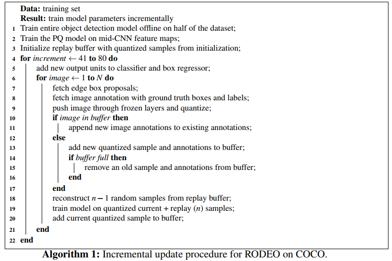
For lifelong learning agents that are required to learn from possibly infinite data streams, it is not possible to store all previous examples in a memory replay buffer. Since the capacity of our memory buffer is fixed, it is essential to replace less useful examples over time. We use a replacement strategy that replaces the image having the least number of unique labels from the replay buffer. We also experiment with other replacement strategies in Sec. 6.1.
对于需要从可能无限的数据流中学习的终身学习代理,不可能将之前的所有示例存储在内存回放缓冲区中。由于内存缓冲区的容量是固定的,因此随着时间的推移,必须更换不太有用的示例。我们使用替换策略来替换重播缓冲区中具有最少唯一标签的图像。我们还在Sec6.1中试验了其他替代策略。
5 实验设置
5.1 Datasets
We use the Pascal VOC 2007 [10] and Microsoft COCO [32] datasets. VOC contains 20 object classes with 5,000 combined training/validation images and 5,000 testing images. COCO contains 80 classes (including all VOC classes) with 80K training images and 40K validation images, which we use for testing. We use the entire validation set as our test set.
我们使用Pascal VOC 2007【10】和Microsoft COCO【32】数据集。VOC包含20个对象类,包含5000个组合训练/验证图像和5000个测试图像。COCO包含80个类(包括所有VOC类),包含80K训练图像和40K验证图像,我们使用这些图像进行测试。我们使用整个验证集作为测试集。
5.2 Baseline Models
We compare several baselines using the Fast RCNN architecture with edge box proposals and a ResNet-50 [18] backbone, which is the setup used in [51]. These baselines include:
• RODEO – RODEO operates as an incremental object detector by using replay mechanisms to mitigate forgetting. Our main variant replays 4 randomly selected samples from its buffer at each time step. We use 32 codebooks for VOC and 64 for COCO, each of size 256.
• Fine-Tune (No Replay) – This is a standard object detection model without a replay buffer that is fine-tuned one example at a time with only a single epoch through the dataset. This model serves as a lower bound on performance and suffers from catastrophic forgetting of previous classes.
• ILwFOD – The Incremental Learning without Forgetting Object Detection model [51] uses a fixed proposal generator (e.g., edge boxes) with distillation to incrementally learn classes. It is the current state-of-the-art for incremental object detection.
• SLDA + Stream-Regress – Deep streaming linear discriminant analysis was recently shown to work well in classifying deep network features on ImageNet [15]. Since SLDA is only used for classification, we combine it with a streaming regression model to regress for bounding box coordinates. To handle the background class with SLDA, we store a mean vector per class and a background mean vector per class, along with a universal covariance matrix. At test time, a label is assigned based on the closest Gaussian in feature space, defined by the class mean vectors and universal covariance matrix. More details for this model are provided in supplemental materials.
• Offline – This is a standard object detection network trained in the offline setting using mini-batches and multiple epochs through the dataset. This model serves as an upper bound for our experiments.
我们比较了使用Faster RCNN体系结构、边界框方案和ResNet-50骨干网(即[51]中使用的设置)的多条基线。这些基线包括:
•RODEO–RODEO作为一个增量目标检测器,通过使用回放机制来缓解遗忘。我们的主要变体在每个时间步从缓冲区中重放4个随机选择的样本。我们对VOC使用32个码本,COCO使用64个码本,每个码本的大小为256。
•微调(无回放)-这是一种标准的目标检测模型,没有回放缓冲区,每次微调一个示例,数据集中只有一个历元。该模型作为性能的下界,并遭受对以前类的灾难性遗忘。
•ILwFOD–不忘目标检测的增量学习模型【51】使用带有蒸馏的固定建议生成器(如边缘框)来增量学习类。这是目前最先进的增量目标检测技术。
•SLDA+流回归–深流线性判别分析最近被证明可以很好地对ImageNet上的深层网络特征进行分类【15】。由于SLDA仅用于分类,我们将其与流式回归模型相结合,对边界框坐标进行回归。为了使用SLDA处理背景类,我们存储了每个类的平均向量和每个类的背景平均向量,以及通用协方差矩阵。在测试时,根据类平均向量和通用协方差矩阵定义的特征空间中最近的高斯分布分配标签。补充材料中提供了该模型的更多详细信息。
•离线-这是一个标准的目标检测网络,在离线设置下通过数据集使用小批量和多个epoch进行训练。这个模型为我们的实验提供了一个上限。
All models use the same network initialization procedure. Similarly, all models are optimized with stochastic gradient descent with momentum, except SLDA. We were not able to replicate the results for ILwFOD, so we use the numbers provided by the authors for VOC and do not include results for COCO since our setup differs. While RODEO, LDA+Stream-Regress, and Fine-Tune are all streaming models trained one sample at a time with a single epoch through the dataset, ILwFOD is an incremental batch method that loops through batches of data many times making it less ideal for immediate learning.
所有型号都使用相同的网络初始化过程。同样,除SLDA外,所有模型均采用带动量的随机梯度下降法进行优化。我们无法复制ILwFOD的结果,因此我们使用作者提供的VOC数据,不包括COCO的结果,因为我们的设置不同。虽然RODEO、LDA+Stream Retression和Fine Tune都是通过数据集以单个历元一次训练一个样本的流模型,但ILwFOD是一种增量批处理方法,多次循环处理数据批,因此不太适合立即学习。
5.3 Metrics
We introduce a new metric that captures a model’s mean average precision (mAP) at a 0.5 IoU threshold over time. This metric extends the Wall metric from [16, 26] for object detection and normalizes an incremental learner’s performance to an optimized offline baseline, i.e., ![]() ; where at is an incremental learner’s mAP at time t,
; where at is an incremental learner’s mAP at time t, ![]() is the offline learner’s mAP at time t, and there are T total testing events. We only evaluate performance on classes learned until time t. While
is the offline learner’s mAP at time t, and there are T total testing events. We only evaluate performance on classes learned until time t. While ![]() is usually between 0 and 1, a value greater than 1 is possible if the incremental learner performed better than the offline baseline. This metric makes it easier to compare performance across datasets of varying difficulty.
is usually between 0 and 1, a value greater than 1 is possible if the incremental learner performed better than the offline baseline. This metric makes it easier to compare performance across datasets of varying difficulty.
我们引入了一个新的度量,它可以捕获模型在0.5 IoU阈值下随时间变化的平均精度(mAP)。该度量将目标检测的墙度量从[16,26]扩展到了优化的离线基线,即![]() ;其中at是时间t的增量学习器mAP,
;其中at是时间t的增量学习器mAP,![]() ;t是时间t的离线学习器mAP,总共有t个测试事件。我们只评估在时间t之前学习的类别的表现。虽然
;t是时间t的离线学习器mAP,总共有t个测试事件。我们只评估在时间t之前学习的类别的表现。虽然![]() 通常在0到1之间,但如果增量学习者的表现优于离线基线,则该值可能大于1。此指标使比较不同难度数据集的性能变得更加容易。
通常在0到1之间,但如果增量学习者的表现优于离线基线,则该值可能大于1。此指标使比较不同难度数据集的性能变得更加容易。
5.4 Training Protocol
In our training paradigm, the model is first initialized with half the total classes and then it is required to learn the second half of the dataset one class at a time, which follows the setup in [51]. We organize the classes in alphabetical order for both PASCAL VOC 2007 and COCO. For example, on VOC, which contains 20 total classes, the network is first initialized with classes 1-10, and then the network learns class 11, then 12, then 13, etc. This paradigm closely matches how incremental class learning experiments have been performed for classification tasks [17, 44]. For all experiments, the network is incrementally trained on all images containing at least one instance for the new class. This means that images could potentially be repeated in previous or future increments. When training a new class, only the labels for the ground truth boxes containing that particular class are provided.
在我们的训练范式中,首先用总类数的一半初始化模型,然后需要一次学习数据集的后半部分,一次学习一个类,这遵循了[51]中的设置。我们按照帕斯卡VOC 2007和COCO的字母顺序组织课程。例如,在总共包含20个类的VOC上,首先用类1-10初始化网络,然后网络学习类11,然后是12,然后是13,等等。这种范式与分类任务的增量类学习实验的执行方式非常匹配【17,44】。对于所有实验,网络都会在包含至少一个新类实例的所有图像上进行增量训练。这意味着图像可能会以以前或将来的增量重复。训练新类别时,仅提供包含该特定类别的ground truth的标签。
For incremental batch models, after base initialization, models are provided a batch containing all data for a single class, which they are allowed to loop over. Streaming models operate on the same batches of data, but examples from within the batch are observed one at a time and can only be observed once, unless the data is cached in a memory buffer. For VOC, after each new class is learned, each model is evaluated on test data containing at least one box of any previously trained classes. For COCO, models are updated on batches containing a single class after base initialization, which is identical to the VOC paradigm. However, since COCO is much larger than VOC and evaluation takes much longer, we evaluate the model after every 10 new classes of data have been trained.
对于增量批处理模型,在基本初始化之后,将为模型提供一个包含单个类的所有数据的批处理,允许模型循环。流模型对相同批次的数据进行操作,但批次内的示例一次只能观察一次,除非数据缓存在内存缓冲区中。对于VOC,在学习每个新类后,将根据包含至少一个先前训练类框的测试数据对每个模型进行评估。对于COCO,在基类初始化之后,在包含单个类的批上更新模型,这与VOC范式相同。然而,由于COCO比VOC大得多,评估需要更长的时间,我们在每10类新数据经过训练后评估模型。
5.5 Implementation Details
Following [51], we use the Fast RCNN architecture [55] with a ResNet-50 [18] backbone and edge box object proposals [59] for all models, unless otherwise noted. Edge boxes is an unsupervised method for producing class agnostic object proposals, which is useful in the streaming setting where we don’t know what types of objects will appear in future time steps. Specifically, we compute 2,000 edge boxes for an image. Following [48], we first resize images to 800 × 1000 pixels. To determine whether a box should be labelled as background or foreground, we compute overlap with ground truth boxes using an IoU threshold of 0.5. Then, batches of 64 boxes are randomly selected per image, where each batch must have roughly 25% positive boxes (IoU > 0.5). During inference, 128 boxes are chosen as output after applying a per-category Non-Maximal Supression (NMS) threshold of 0.3 to eliminate overlapping boxes. More parameter settings are in supplemental materials.
在【51】之后,除非另有说明,否则我们使用Faster RCNN体系结构【55】以及所有模型的ResNet-50【18】主干和边缘框目标方案【59】。边缘框是一种无监督的方法,用于生成与类无关的目标建议,这在流式处理设置中很有用,因为我们不知道未来的时间步长中将出现什么类型的对象。具体来说,我们为一幅图像计算2000个边缘框。在[48]之后,我们首先将图像大小调整为800×1000像素。为了确定框是否应标记为背景或前景,我们使用IoU阈值0.5计算与地面真实框的重叠。然后,每个图像随机选择64个盒子的批次,其中每个批次必须有大约25%的正样本框(IoU>0.5)。在推理过程中,在应用0.3的每类非最大抑制(NMS)阈值以消除重叠框后,选择128个框作为输出。补充资料中提供了更多参数设置。
For each input image to RODEO, layer G produces feature map tensors of approximate size 25 × 30 × 2048. Images from the base initialization classes (1-10) for VOC and (1-40) for COCO are used to train the PQ model. For VOC, we are able to fit all the feature maps in memory to train the PQ model. For COCO, it is not possible to fit all the images in memory, so we sub-sample 30 random locations from the full feature map of each image to train the PQ. The ResNet-50 backbone has four residual blocks. We quantize RODEO after the third residual block, i.e., F consists of the last residual block, the Fast RCNN MLP head composed of two fully connected layers, and the linear classifier and regressor. To make experiments fair, we subject RODEO’s replay buffer to an upper limit of 510 MB, which is the amount of memory required by ILwFOD. For VOC, this allows RODEO to store a representation of every sample in the training set. For COCO, this only allows us to store 17,668 compressed samples. To manage the buffer, we use a strategy that always replaces the image with the least number of unique objects.
对于RODEO的每个输入图像,图层G生成大约大小为25×30×2048的特征地图张量。VOC的基本初始化类(1-10)和COCO的基本初始化类(1-40)的图像用于训练PQ模型。对于VOC,我们能够拟合内存中的所有特征映射来训练PQ模型。对于COCO来说,不可能在内存中匹配所有图像,因此我们从每个图像的全特征图中随机抽取30个位置来训练PQ。ResNet-50主干有四个剩余块。我们在第三个残差块之后对RODEO进行量化,即F由最后一个残差块、由两个完全连接的层组成的Fast RCNN MLP头以及线性分类器和回归器组成。为了公平起见,我们将RODEO的重播缓冲区设置为510 MB的上限,这是ILwFOD所需的内存量。对于VOC,这允许RODEO存储训练集中每个样本的表示。对于COCO,这只允许我们存储17668个压缩样本。为了管理缓冲区,我们使用一种策略,总是用最少数量的唯一目标替换图像。
6 实验结果
Our main experimental results are in Table 1and learning curves are in Fig. 2 and Fig. 3 for VOC and COCO, respectively. We include results for RODEO models that use both real and reconstructed features. Real features do not undergo reconstruction before being passed through plastic layers, F. To normalize WmAP, we use offline models that achieve final mAP values of 0.715 and 0.42 on VOC and COCO, respectively. Additional results are in supplemental materials.
我们的主要实验结果如表1所示,VOC和COCO的学习曲线分别如图2和图3所示。我们包括使用真实和重建特征的RODEO模型的结果。真实特征在通过层F之前不会进行重建。为了规范化WmAP,我们使用离线模型,在VOC和COCO上分别获得0.715和0.42的最终贴图值。补充材料中有其他结果。
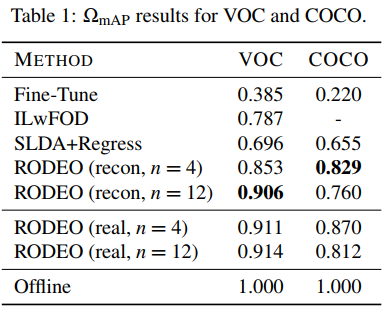
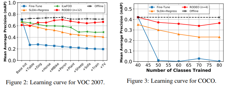
For VOC, RODEO beats all previous methods just by replaying only four samples. Our method is much less prone to forgetting than other models, which is demonstrated by its performance at the final time step in Fig. 2. The SLDA+Regress model is surprisingly competitive on both datasets without the need to update its backbone. For COCO, RODEO is run with four replay samples and outperforms the baseline models by a large margin. Further, across various replay sizes and replacement strategies (Table 2), we find that real features yield better results compared to reconstructed features.
对于VOC,RODEO仅通过重放四个样本就击败了所有以前的方法。与其他模型相比,我们的方法更不容易遗忘,这从图2中最后一个时间步的性能可以看出。SLDA+回归模型在两个数据集上都具有惊人的竞争力,无需更新其主干。对于COCO来说,RODEO有四个重播样本,其表现大大优于基准模型。此外,在各种重播大小和替换策略(表2)中,我们发现真实特征比重建特征产生更好的结果。
To study the impact of the buffer management strategy chosen, we run the following replacement strategies on the COCO dataset. Results are in Table 2.
• BAL: Balanced replacement strategy that replaces the item which least affects the overall class distribution.
• MIN, MAX: Replace the image having the least and highest number of unique labels respectively.
• RANDOM: Randomly replace an image from the buffer.
• NO-REPLACE: No replacement, i.e., store everything and let the buffer expand infinitely.
为了研究所选缓冲区管理策略的影响,我们在COCO数据集上运行以下替换策略。结果见表2。
•BAL:平衡替换策略,替换对整体班级分布影响最小的项目。
•最小、最大:分别替换唯一标签数量最少和最多的图像。
•随机:随机替换缓冲区中的图像。
•无替换:无替换,即存储所有内容并让缓冲区无限扩展。
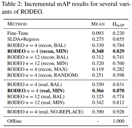
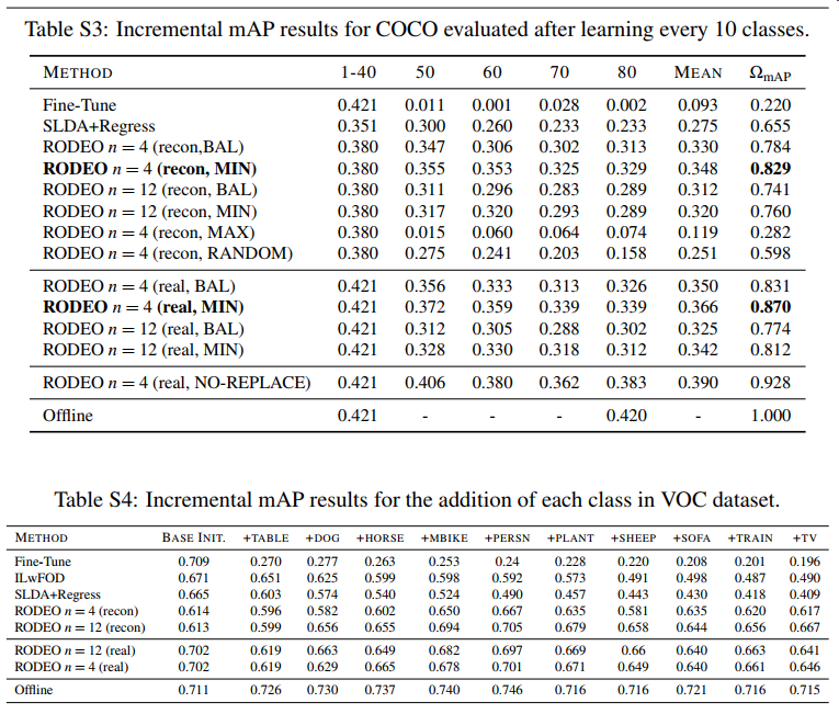
For an ideal case, we ran a version of RODEO with real features (n = 4) and an unlimited buffer (storing everything). This model achieved an WmAP of 0.928. All other replacement strategies are only allowed to store 17,668 samples. We find that MAX replace yields even worse results compared to RANDOM replace suggesting storing more samples with more unique categories is better. Similarly, we find that MIN replace performs better across both real and reconstructed features, even beating the balanced (BAL) replacement strategy. We hypothesize that since MIN replace keeps images with the most unique objects, it results in a more diverse buffer to overcome forgetting.
在理想情况下,我们运行了一个具有真实功能(n=4)和无限缓冲区(存储所有内容)的RODEO版本。该模型的WmAP为0.928。所有其他替换策略仅允许存储17668个样本。我们发现,与随机替换相比,最大替换产生的结果更差,这表明存储更多具有更独特类别的样本更好。同样,我们发现最小替换在真实特征和重构特征上都表现得更好,甚至优于平衡(BAL)替换策略。我们假设,由于MIN-replace将图像保留为最独特的对象,因此它会产生更多样化的缓冲区来克服遗忘。
For our VOC experiments, we do not replace anything from the buffer. As we increase the number of replay samples from 4 to 12, the performance improves by 0.3% for real features and 5.3% for reconstructed features respectively. Surprisingly for COCO, which has buffer replacement, the performance decreases as we increase the number of replay samples. We suspect this could be because COCO has many more objects per image compared to VOC which are being treated as background for region proposal selection. In the future, it would be interesting to develop new methods to handle this background class in an incremental setting, which has been explored for incremental semantic segmentation [5]
对于我们的VOC实验,我们不替换缓冲区中的任何东西。当我们将回放样本数从4个增加到12个时,对于真实特征和重构特征,性能分别提高了0.3%和5.3%。令人惊讶的是,对于具有缓冲区替换的COCO来说,随着重播样本数的增加,性能会下降。我们怀疑这可能是因为COCO与VOC相比,每张图像有更多的目标,而VOC被视为区域建议选择的背景。在未来,开发新的方法以增量方式处理这个背景类将是一件有趣的事情,这已经为增量语义分割进行了探索
6.2 Training Time
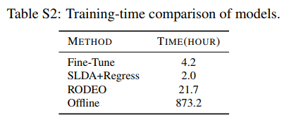
For COCO, we train each incremental iteration of Fast R-CNN for 10 epochs which takes about 21.83 hours. Thus, full offline training of 40 iterations takes a total of 873 hrs. In contrast, our method, RODEO, requires only 22 hours which is a 40× speed-up compared to offline. SLDA+Regress and Fine-Tune both train faster, but perform much worse in terms of detection performance. These numbers do not include the base initialization time, which is the same for all methods. Exact numbers are in supplemental materials (Table S2).
对于COCO,我们对Fast R-CNN的每一次增量迭代进行了10个阶段的训练,大约需要21.83小时。因此,40次迭代的完整离线训练总共需要873小时。相比之下,我们的RODEO方法只需要22小时,与离线相比,这是40倍的速度。SLDA+回归和微调都训练得更快,但检测性能要差得多。这些数字不包括基本初始化时间,这对于所有方法都是相同的。具体数字见补充材料(表S2)。
7 讨论
In current object detection problem formulations, detected objects are not aware of each other. However, many real-world applications require an understanding of attributes and the relationships between objects. For example, Visual Query Detection (VQD) is a new visual grounding task for localizing multiple objects in an image that satisfies a given language query [2]. Our method can be easily extended for the VQD task by modifying the object detector to output only the boxes relevant to the language query.
在当前的目标检测问题公式中,检测到的目标彼此都不知道。然而,许多实际应用程序需要了解属性和目标之间的关系。例如,视觉查询检测(VQD)是一项新的视觉基础任务,用于定位满足给定语言查询的图像中的多个目标[2]。通过修改目标检测器,只输出与语言查询相关的框,我们的方法可以很容易地扩展到VQD任务。
In any real system where memory is limited, the choice of an ideal buffer replacement strategy is vital. For any agent that needs to learn new information over time, while also recalling previous knowledge, it is critical to store the most informative memories and replace those which carry less information. This procedure has also been studied in the reinforcement learning literature as experience replay [22, 31]. Our buffer size is limited because it is calculated with respect to the maximum storage required by the ILwFOD model [51]. To efficiently use this limited storage, we tried various replacement strategies to store the newer examples such as: random replacement, class distribution balancing, and replacement of images with the most or fewest number of unique bounding boxes present. In the future, more efficient strategies for determining the maximum buffer size and replacement strategy could be useful for online applications.
在任何内存有限的实际系统中,选择理想的缓冲区替换策略至关重要。对于任何需要随着时间推移学习新信息的代理,同时也需要回忆以前的知识,存储信息量最大的内存并替换信息量较少的内存是至关重要的。强化学习文献中也对这一过程进行了研究,将其作为经验回放【22,31】。我们的缓冲区大小是有限的,因为它是根据ILwFOD模型所需的最大存储量来计算的【51】。为了有效地使用这个有限的存储,我们尝试了各种替换策略来存储较新的示例,例如:随机替换、类分布平衡,以及使用最多或最少数量的唯一边界框替换图像。将来,确定最大缓冲区大小的更有效策略和替换策略可能对在线应用程序有用。
RODEO is designed explicitly for streaming applications where real-time inference and overall compute are critical factors, such as robotic or embedded devices. Although RODEO uses Fast-RCNN, a two stage detector, which is slower than single stage detectors like SSD [13, 34] and YOLO [45, 46], single stage approaches could be used to facilitate faster learning and inference. Moreover, RODEO currently uses a ResNet-50 backbone and can only process two images in a single batch. Using a more efficient backbone model like a MobileNet [49] or ShuffleNet [37] architecture would allow the model to run faster with fewer storage requirements. In future work, it would be interesting to study how RODEO could be extended to single-stage detectors by replaying intermediate features and directly using the generated anchors instead of edge box proposals.
RODEO专门为实时推理和整体计算是关键因素的流式应用程序而设计,如机器人或嵌入式设备。虽然RODEO使用了Fast RCNN,这是一种两级检测器,比SSD(13,34)和YOLO(45,46)等单级检测器慢,但可以使用单级方法来促进更快的学习和推理。此外,RODEO目前使用ResNet-50主干网,一批只能处理两幅图像。使用更高效的主干网模型,如MobileNet(49)或ShuffleNet(37)体系结构,可以使模型运行更快,存储需求更少。在未来的工作中,研究RODEO如何通过重放中间特征和直接使用生成的锚而不是边缘框方案扩展到单级探测器将是一件有趣的事情。
Further performance gains could be achieved by using augmentation strategies on the midlevel CNN features. Recently, several augmentation strategies have been designed explicitly for object detection [28, 54, 60] and it would be interesting to explore how they could improve performance within deep feature space for an incremental learning application.
通过在中级CNN功能上使用增强策略,可以进一步提高性能。最近,已经为目标检测明确设计了几种增强策略[28、54、60],探索它们如何在增量学习应用程序的深层特征空间中提高性能将是一件有趣的事情。
8 结论
We proposed RODEO, a new method that pioneers streaming object detection. RODEO uses replay of quantized, mid-level CNN features to mitigate catastrophic forgetting on a fixed memory budget. Using our new model, we achieve state-of-the-art performance for incremental object detection tasks on the PASCAL VOC 2007 and MS COCO datasets when compared against models that operate in the easier incremental batch learning paradigm.
我们提出了RODEO,这是一种开创流式目标检测的新方法。RODEO使用量化的、中级的CNN功能回放,以在固定内存预算下缓解灾难性遗忘。使用我们的新模型,我们在PASCAL VOC 2007和MS COCO数据集上实现了最先进的增量对象检测任务性能,与在更简单的增量批处理学习范式中运行的模型相比。
Furthermore, our model is general enough to be applied to multi-modal incremental detection tasks in the future like VQD [2], which require an agent to understand scenes and the relationships between objects within them
此外,我们的模型具有足够的通用性,可以应用于未来的多模式增量检测任务,如VQD【2】,这需要代理了解场景以及场景中目标之间的关系
附录
S1 Training Details
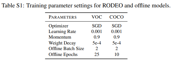
Hyper-parameter settings for RODEO and the offline models for VOC and COCO are given in Table S1. Similarly, run time comparisons for the COCO dataset are in Table S2.
RODEO的超参数设置以及VOC和COCO的离线模型如表S1所示。类似地,COCO数据集的运行时比较见表S2。
S2 Where to Quantize?
Our choices of layers to quantize are limited due to the architecture of the ResNet-50 backbone. ResNet-50 has four main major layers with each having (3,4,6,3) bottleneck blocks respectively. Since bottleneck blocks add a residual shortcut connection at the end, it is not possible to quantize from the middle of the block, leaving only four places to perform quantization. Quantizing earlier has some advantages since it leaves more trainable parameters for the incremental model, which could lead to better results [17]. But, it also requires twice the memory to store the same number of images as we move towards the earlier layers. For efficiency, we choose the last layer for feature quantization.
由于ResNet-50主干的体系结构,我们对量化层的选择受到限制。ResNet-50有四个主要层,每个层分别有(3、4、6、3)个瓶颈块。由于瓶颈块在末尾添加了残差连接,因此不可能从块的中间进行量化,只留下四个位置来执行量化。早期量化有一些优势,因为它为增量模型留下了更多可训练的参数,这可能导致更好的结果【17】。但是,它还需要两倍的内存来存储相同数量的图像,因为我们要向早期的层移动。为了提高效率,我们选择最后一层进行特征量化。
S3 Additional Results
We provide the individual mAP results for each increment of COCO in Table S3 and VOC in Table S4.
我们在表S3中提供了COCO每增加一次的单独mAP结果,在表S4中提供了VOC。
S4 Additional SLDA+Stream-Regress Object Detection Details
An overview of the incremental training stage for the SLDA+Stream-Regress object detection model is given in Alg. 2. We use the Fast RCNN model to extract features from edge box proposals. Given a new input, we then make classification and regression predictions using the SLDA and Stream-Regress models, respectively. For both the SLDA model and the Stream-Regress models, we use shrinkage regularization with parameters of 1e−2 and 1e−4, respectively.
流程2概述了SLDA+流回归目标检测模型的增量训练阶段。我们使用Fast RCNN模型从边缘盒方案中提取特征。在给定新输入的情况下,我们分别使用SLDA和流回归模型进行分类和回归预测。对于SLDA模型和流回归模型,我们使用参数分别为1e−2和1e−4的收缩正则化。
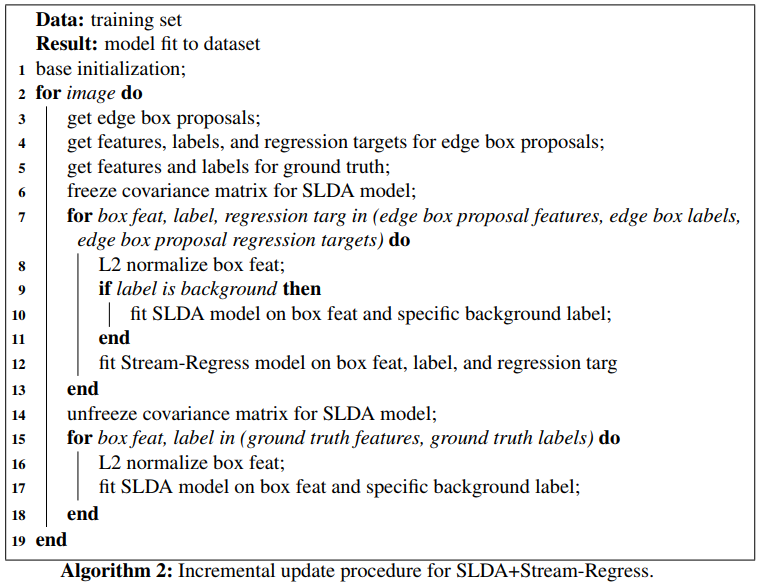
We train the SLDA model as proposed in [15] with one slight modification. In [15], there was a single mean vector stored per class. However, in our work we allow SLDA to store two mean vectors per class, where one mean vector is representative of the actual class data and the second mean vector is representative of the background for that particular class. During test time, we thus obtain two scores for each class: the main class score and the background class score. We keep the main class score for each class and only keep the maximum score of all background scores.
我们对[15]中提出的SLDA模型进行了一次轻微的修改。在【15】中,每个类存储一个平均向量。然而,在我们的工作中,我们允许SLDA为每个类存储两个平均向量,其中一个平均向量代表实际类数据,第二个平均向量代表特定类的背景。在测试期间,我们为每个类别获得了两个分数:主要类别分数和背景类别分数。我们保留每个类别的主要类别分数,只保留所有背景分数的最高分。
Training the Stream-Regress model is similar to training the SLDA model. That is, we first initialize one mean vector ![]() to zeros, where d is the dimension of the data. We initialize another mean vector
to zeros, where d is the dimension of the data. We initialize another mean vector ![]() to zeros, where m is the number of regression targets, and we have four regression coordinates per class including the background class. We also initialize two covariance matrices,
to zeros, where m is the number of regression targets, and we have four regression coordinates per class including the background class. We also initialize two covariance matrices, ![]() , and a total count of the number of updates, N ∈ R.
, and a total count of the number of updates, N ∈ R.
流回归模型的训练与SLDA模型的训练类似。也就是说,我们首先将一个平均向量![]() 初始化为零,其中d是数据的维数。我们将另一个平均向量
初始化为零,其中d是数据的维数。我们将另一个平均向量![]() 初始化为零,其中m是回归目标的数量,我们每个类有四个回归坐标,包括背景类。我们还初始化了两个协方差矩阵,
初始化为零,其中m是回归目标的数量,我们每个类有四个回归坐标,包括背景类。我们还初始化了两个协方差矩阵,![]() ,以及更新总数N∈ R
,以及更新总数N∈ R
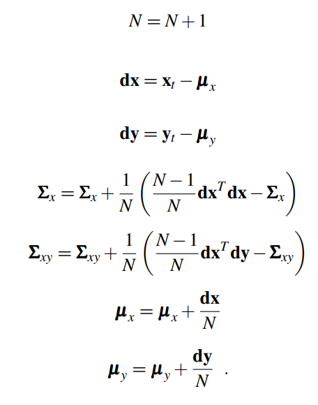
Given a new sample (xt,yt), where![]() is a one-hot encoding of the regression targets, we make the following updates to our model:
is a one-hot encoding of the regression targets, we make the following updates to our model:
给定一个新样本(xt,yt),其中![]() 是回归目标的one-hot编码,我们对模型进行以下更新:
是回归目标的one-hot编码,我们对模型进行以下更新:
To make predictions, we first compute the precision matrix
为了进行预测,我们首先计算精度矩阵
![]()
with shrinkage parameter e and identity matrix ![]() . We then compute regression targets,
. We then compute regression targets,![]() , for an input xt as:
, for an input xt as:
使用收缩参数e和单位矩阵![]() 。然后,我们计算输入xt的回归目标
。然后,我们计算输入xt的回归目标![]() ,如下所示:
,如下所示:
![]()
![]()


 4003
4003

 被折叠的 条评论
为什么被折叠?
被折叠的 条评论
为什么被折叠?
 到【灌水乐园】发言


