智慧交通day02-车流量检测实现05：卡尔曼滤波器实践(小车模型)

1.filterpy

FilterPy是一个实现了各种滤波器的Python模块，它实现著名的卡尔曼滤波和粒子滤波器。我们可以直接调用该库完成卡尔曼滤波器实现。其中的主要模块包括：

• filterpy.kalman

  该模块主要实现了各种卡尔曼滤波器，包括常见的线性卡尔曼滤波器，扩展卡尔曼滤波器等。

• filterpy.common

  该模块主要提供支持实现滤波的各种辅助函数，其中计算噪声矩阵的函数，线性方程离散化的函数等。

• filterpy.stats

  该模块提供与滤波相关的统计函数，包括多元高斯算法，对数似然算法，PDF及协方差等。

• filterpy.monte_carlo

  该模块提供了马尔科夫链蒙特卡洛算法，主要用于粒子滤波。

开源代码在：

https://github.com/rlabbe/filterpy/tree/master/filterpy/kalman

我们介绍下卡尔曼滤波器的实现，主要分为预测和更新两个阶段，在进行滤波之前，需要先进行初始化：

• 初始化

预先设定状态变量dim_x和观测变量维度dim_z、协方差矩阵P、运动形式和观测矩阵H等，一般各个协方差矩阵都会初始化为单位矩阵，根据特定的场景需要相应的设置。

def __init__(self, dim_x, dim_z, dim_u = 0, x = None, P = None,
             Q = None, B = None, F = None, H = None, R = None):
    """Kalman Filter
        Refer to http:/github.com/rlabbe/filterpy

        Method
        -----------------------------------------
         Predict        |        Update
        -----------------------------------------
                        |  K = PH^T(HPH^T + R)^-1
        x = Fx + Bu     |  y = z - Hx
        P = FPF^T + Q   |  x = x + Ky
                        |  P = (1 - KH)P
                        |  S = HPH^T + R
        -----------------------------------------
        note: In update unit, here is a more numerically stable way: P = (I-KH)P(I-KH)' + KRK'

        Parameters
        ----------
        dim_x: int
            dims of state variables, eg:(x,y,vx,vy)->4
        dim_z: int
            dims of observation variables, eg:(x,y)->2
        dim_u: int
            dims of control variables,eg: a->1
            p = p + vt + 0.5at^2
            v = v + at
            =>[p;v] = [1,t;0,1][p;v] + [0.5t^2;t]a
        """

    assert dim_x >= 1, 'dim_x must be 1 or greater'
    assert dim_z >= 1, 'dim_z must be 1 or greater'
    assert dim_u >= 0, 'dim_u must be 0 or greater'

    self.dim_x = dim_x
    self.dim_z = dim_z
    self.dim_u = dim_u

    # initialization
    # predict
    self.x = np.zeros((dim_x, 1)) if x is None else x      # state
    self.P = np.eye(dim_x)  if P is None else P            # uncertainty covariance
    self.Q = np.eye(dim_x)  if Q is None else Q            # process uncertainty for prediction
    self.B = None if B is None else B                      # control transition matrix
    self.F = np.eye(dim_x)  if F is None else F            # state transition matrix

    # update
    self.H = np.zeros((dim_z, dim_x)) if H is None else H  # Measurement function z=Hx
    self.R = np.eye(dim_z)  if R is None else R            # observation uncertainty
    self._alpha_sq = 1.                              # fading memory control
    self.z = np.array([[None] * self.dim_z]).T       # observation
    self.K = np.zeros((dim_x, dim_z))                # kalman gain
    self.y = np.zeros((dim_z, 1))                    # estimation error
    self.S = np.zeros((dim_z, dim_z))                # system uncertainty, S = HPH^T + R
    self.SI = np.zeros((dim_z, dim_z))               # inverse system uncertainty, SI = S^-1

    self.inv = np.linalg.inv
    self._mahalanobis = None                         # Mahalanobis distance of measurement
    self.latest_state = 'init'                       # last process name

• 预测阶段

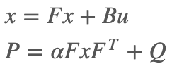
接下来进入预测环节，为了保证通用性，引入了遗忘系数α，其作用在于调节对过往信息的依赖程度，α越大对历史信息的依赖越小：

 代码如下：

def predict(self, u = None, B = None, F = None, Q = None):
    """
    Predict next state (prior) using the Kalman filter state propagation equations:
                         x = Fx + Bu
                         P = fading_memory*FPF^T + Q

    Parameters
    ----------

    u : ndarray
        Optional control vector. If not `None`, it is multiplied by B
        to create the control input into the system.

    B : ndarray of (dim_x, dim_z), or None
        Optional control transition matrix; a value of None
        will cause the filter to use `self.B`.

    F : ndarray of (dim_x, dim_x), or None
        Optional state transition matrix; a value of None
        will cause the filter to use `self.F`.

    Q : ndarray of (dim_x, dim_x), scalar, or None
        Optional process noise matrix; a value of None will cause the
        filter to use `self.Q`.
    """

    if B is None:
        B = self.B
    if F is None:
        F = self.F
    if Q is None:
        Q = self.Q
    elif np.isscalar(Q):
        Q = np.eye(self.dim_x) * Q

    # x = Fx + Bu
    if B is not None and u is not None:
        self.x = F @ self.x + B @ u
    else:
        self.x = F @ self.x

    # P = fading_memory*FPF' + Q
    self.P = self._alpha_sq * (F @ self.P @ F.T) + Q
    self.latest_state = 'predict'

• 更新阶段

按下式进行状态的更新：

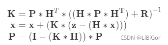
 也可以写为：

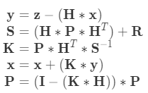
 其中，y是测量余量，S是测量余量的协方差矩阵。

在实际应用中会做一些微调，使协方差矩阵为：

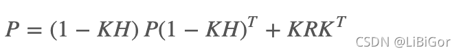
代码如下：

def update(self, z, R = None, H = None):
    """
    Update Process, add a new measurement (z) to the Kalman filter.
                K = PH^T(HPH^T + R)^-1
                y = z - Hx
                x = x + Ky
                P = (1 - KH)P or P = (I-KH)P(I-KH)' + KRK'

    If z is None, nothing is computed.

    Parameters
    ----------
    z : (dim_z, 1): array_like
        measurement for this update. z can be a scalar if dim_z is 1,
        otherwise it must be convertible to a column vector.

    R : ndarray, scalar, or None
        Optionally provide R to override the measurement noise for this
        one call, otherwise  self.R will be used.

    H : ndarray, or None
        Optionally provide H to override the measurement function for this
        one call, otherwise self.H will be used.
    """

    if z is None:
        self.z = np.array([[None] * self.dim_z]).T
        self.y = np.zeros((self.dim_z, 1))
        return

    z = reshape_z(z, self.dim_z, self.x.ndim)

    if R is None:
        R = self.R
    elif np.isscalar(R):
        R = np.eye(self.dim_z) * R

    if H is None:
        H = self.H

    if self.latest_state == 'predict':
        # common subexpression for speed
        PHT = self.P @ H.T

        # S = HPH' + R
        # project system uncertainty into measurement space
        self.S = H @ PHT + R

        self.SI = self.inv(self.S)


        # K = PH'inv(S)
        # map system uncertainty into kalman gain
        self.K = PHT @ self.SI

        # P = (I-KH)P(I-KH)' + KRK'
        # This is more numerically stable and works for non-optimal K vs
        # the equation P = (I-KH)P usually seen in the literature.
        I_KH = np.eye(self.dim_x) - self.K @ H
        self.P = I_KH @ self.P @ I_KH.T + self.K @ R @ self.K.T


    # y = z - Hx
    # error (residual) between measurement and prediction
    self.y = z - H @ self.x

    self._mahalanobis = math.sqrt(float(self.y.T @ self.SI @ self.y))

    # x = x + Ky
    # predict new x with residual scaled by the kalman gain

    self.x = self.x + self.K @ self.y
    self.latest_state = 'update'

那接下来，我们就是用filterpy中的卡尔曼滤波器方法完成小车位置的预测。

2.小车案例

现在利用卡尔曼滤波对小车的运动状态进行预测。主要流程如下所示：

• 导入相应的工具包
• 小车运动数据生成
• 参数初始化
• 利用卡尔曼滤波进行小车状态预测
• 可视化：观察参数的变化与结果

下面我们看下整个流程实现：

• 导入包

from matplotlib import pyplot as plt
import seaborn as sns
import numpy as np
from filterpy.kalman import KalmanFilter

• 小车运动数据生成

在这里我们假设小车作速度为1的匀速运动

# 生成1000个位置，从1到1000，是小车的实际位置
z = np.linspace(1,1000,1000) 
# 添加噪声
mu,sigma = 0,1
noise = np.random.normal(mu,sigma,1000)
# 小车位置的观测值
z_nosie = z+noise

• 参数初始化

# dim_x 状态向量size,在该例中为[p,v]，即位置和速度,size=2
# dim_z 测量向量size，假设小车为匀速，速度为1，测量向量只观测位置，size=1
my_filter = KalmanFilter(dim_x=2, dim_z=1)

# 定义卡尔曼滤波中所需的参数
# x 初始状态为[0,0],即初始位置为0，速度为0.
# 这个初始值不是非常重要，在利用观测值进行更新迭代后会接近于真实值
my_filter.x = np.array([[0.], [0.]])

# p 协方差矩阵，表示状态向量内位置与速度的相关性
# 假设速度与位置没关系，协方差矩阵为[[1,0],[0,1]]
my_filter.P = np.array([[1., 0.], [0., 1.]])

# F 初始的状态转移矩阵，假设为匀速运动模型，可将其设为如下所示
my_filter.F = np.array([[1., 1.], [0., 1.]])

# Q 状态转移协方差矩阵，也就是外界噪声，
# 在该例中假设小车匀速，外界干扰小，所以我们对F非常确定，觉得F一定不会出错，所以Q设的很小
my_filter.Q = np.array([[0.0001, 0.], [0., 0.0001]])

# 观测矩阵 Hx = p
# 利用观测数据对预测进行更新，观测矩阵的左边一项不能设置成0
my_filter.H = np.array([[1, 0]])
# R 测量噪声，方差为1
my_filter.R = 1

• 卡尔曼滤波进行预测

# 保存卡尔曼滤波过程中的位置和速度
z_new_list = []
v_new_list = []
# 对于每一个观测值，进行一次卡尔曼滤波 
for k in range(len(z_nosie)):
    # 预测过程 
    my_filter.predict()
    # 利用观测值进行更新
    my_filter.update(z_nosie[k])
    # do something with the output
    x = my_filter.x
    # 收集卡尔曼滤波后的速度和位置信息
    z_new_list.append(x[0][0])
    v_new_list.append(x[1][0])

• 可视化

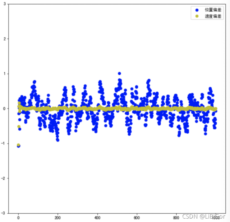
• 预测误差的可视化

  # 位移的偏差
  dif_list = []
  for k in range(len(z)):
      dif_list.append(z_new_list[k]-z[k])
  # 速度的偏差
  v_dif_list = []
  for k in range(len(z)):
      v_dif_list.append(v_new_list[k]-1)
  plt.figure(figsize=(20,9))
  plt.subplot(1,2,1)
  plt.xlim(-50,1050)
  plt.ylim(-3.0,3.0)
  plt.scatter(range(len(z)),dif_list,color ='b',label = "位置偏差")
  plt.scatter(range(len(z)),v_dif_list,color ='y',label = "速度偏差")
  plt.legend()

  运行结果如下所示：

2.卡尔曼滤波器参数的变化

首先定义方法将卡尔曼滤波器的参数堆叠成一个矩阵，右下角补0，我们看一下参数的变化。

# 定义一个方法将卡尔曼滤波器的参数堆叠成一个矩阵，右下角补0 
def filter_comb(p, f, q, h, r):
        a = np.hstack((p, f))
        b = np.array([r, 0])
        b = np.vstack([h, b])
        b = np.hstack((q, b))
        a = np.vstack((a, b))
        return a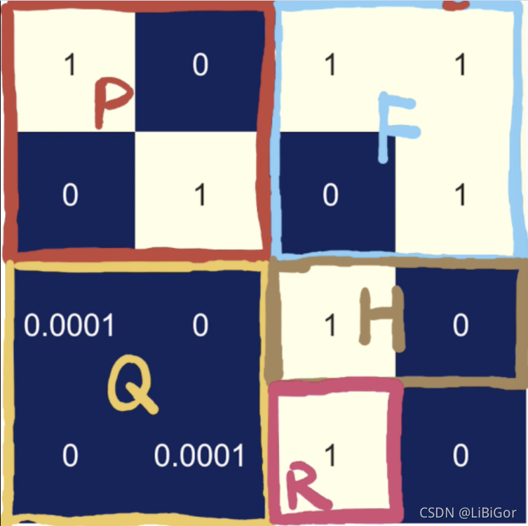

 对参数变化进行可视化：

# 保存卡尔曼滤波过程中的位置和速度
z_new_list = []
v_new_list = []
# 对于每一个观测值，进行一次卡尔曼滤波 
for k in range(1):
    # 预测过程 
    my_filter.predict()
    # 利用观测值进行更新
    my_filter.update(z_nosie[k])
    # do something with the output
    x = my_filter.x
    c = filter_comb(my_filter.P,my_filter.F,my_filter.Q,my_filter.H,my_filter.R)
    plt.figure(figsize=(32,18))
    sns.set(font_scale=4)
    #sns.heatmap(c,square=True,annot=True,xticklabels=False,yticklabels==False,cbar=False)
    sns.heatmap(c,square=True,annot=True,xticklabels=False,yticklabels=False,cbar=False)

对比变换：

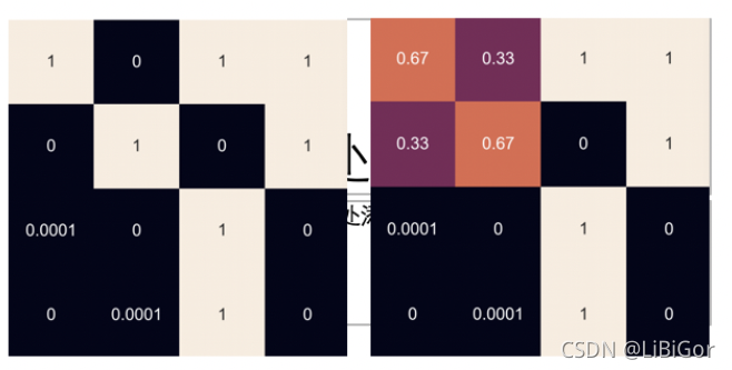
从图中可以看出变化的P，其他的参数F，Q，H,R为变换。另外状态变量x和卡尔曼系数K也是变化的。

3.概率密度函数

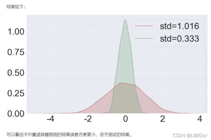
为了验证卡尔曼滤波的结果优于测量的结果，绘制预测结果误差和测量误差的概率密度函数：

# 生成概率密度图像
z_noise_list_std = np.std(noise)
z_noise_list_avg = np.mean(noise)
z_filterd_list_std = np.std(dif_list)
import seaborn as sns 
plt.figure(figsize=(16,9))
ax = sns.kdeplot(noise,shade=True,color="r",label="std=%.3f"%z_noise_list_std)
ax = sns.kdeplot(dif_list,shade=True,color="g",label="std=%.3f"%z_filterd_list_std)

结果如下：

---

总结：

1.了解filterpy工具包

FilterPy是一个实现了各种滤波器的Python模块，它实现著名的卡尔曼滤波和粒子滤波器。直接调用该库完成卡尔曼滤波器实现。

2.知道卡尔曼滤波的实现过程

卡尔曼滤波器的实现，主要分为预测和更新两个阶段，在进行滤波之前，需要先进行初始化

• 初始化

预先设定状态变量和观测变量维度、协方差矩阵、运动形式和转换矩阵

• 预测

对状态变量X和协方差P进行预测

• 更新

利用观测结果对卡尔曼滤波的结果进行修征

3.能够利用卡尔曼滤波器完成小车目标状态的预测

• 导入相应的工具包

• 小车运动数据生成：匀速运动的小车模型

• 参数初始化：对卡尔曼滤波的参数进行初始化，包括状态变量和观测变量维度、协方差矩阵、运动形式和转换矩阵等

• 利用卡尔曼滤波进行小车状态预测：使用Filterpy工具包，调用predict和update完成小车状态的预测

• 可视化：观察参数的变化与结果

  1.预测误差的分布：p,v

  2.参数的变化：参数中变化的是X，P，K，不变的是F，Q，H，R

  1. 误差的概率密度函数：卡尔曼预测的结果优于测量结果