


零基础入门数据挖掘-Task2 数据分析
本文为参加数据挖掘比赛第二阶段的心得分享。
Datawhale 二手车数据挖掘-Task2数据分析
一、 EDA-Exploratory Data Analysis-数据探索性分析
任务目标:
EDA的价值主要在于熟悉数据集,了解数据集,对数据集进行验证来确定所获得数据集可以用于接下来的机器学习或者深度学习使用。
当了解了数据集之后我们下一步就是要去了解变量间的相互关系以及变量与预测值之间的存在关系。
引导数据科学从业者进行数据处理以及特征工程的步骤,使数据集的结构和特征集让接下来的预测问题更加可靠。
完成对于数据的探索性分析,并对于数据进行一些图表或者文字总结并打卡。
二、 相关任务
1.载入各种数据科学以及可视化库:
数据科学库 pandas、numpy、scipy;
可视化库 matplotlib、seabon;其他;
2.载入数据:
载入训练集和测试集;
简略观察数据(head()+shape);
3.数据总览:
通过describe()来熟悉数据的相关统计量
通过info()来熟悉数据类型
4.判断数据缺失和异常
查看每列的存在nan情况
异常值检测
5.了解预测值的分布
总体分布概况(无界约翰逊分布等)
查看skewness and kurtosis
查看预测值的具体频数
6.特征分为类别特征和数字特征,并对类别特征查看unique分布
7.数字特征分析
相关性分析
查看几个特征得 偏度和峰值
每个数字特征得分布可视化
数字特征相互之间的关系可视化
多变量互相回归关系可视化
8.类型特征分析
unique分布
类别特征箱形图可视化
类别特征的小提琴图可视化
类别特征的柱形图可视化类别
特征的每个类别频数可视化(count_plot)
9.用pandas_profiling生成数据报告
三、 对应代码实现
1.载入各种数据科学以及可视化库: 数据科学库 pandas、numpy、scipy; 可视化库 matplotlib、seabon;其他;#coding:utf-8
#导入warnings包,利用过滤器来实现忽略警告语句。
import warnings
warnings.filterwarnings('ignore')

import pandas as pd
import numpy as np
import matplotlib.pyplot as plt
import seaborn as sns
import missingno as msno
2.载入数据:
##载入训练集和测试集;
##简略观察数据(head()+shape);
## 1) 载入训练集和测试集;
Train_data = pd.read_csv('data/car_train_0110.csv', sep=' ')
Test_data = pd.read_csv('data/car_testA_0110.csv', sep=' ')
输出首尾5行,对于观察数据的大概特征很方便
## 2) 简略观察数据(head()+shape)
Train_data.head().append(Train_data.tail())
| SaleID | name | regDate | model | brand | bodyType | fuelType | gearbox | power | kilometer | ... | v_14 | v_15 | v_16 | v_17 | v_18 | v_19 | v_20 | v_21 | v_22 | v_23 | |
|---|---|---|---|---|---|---|---|---|---|---|---|---|---|---|---|---|---|---|---|---|---|
| 0 | 134890 | 734 | 20160002 | 13.0 | 9 | NaN | 0.0 | 1.0 | 0 | 15.0 | ... | 0.092139 | 0.000000 | 18.763832 | -1.512063 | -1.008718 | -12.100623 | -0.947052 | 9.077297 | 0.581214 | 3.945923 |
| 1 | 306648 | 196973 | 20080307 | 72.0 | 9 | 7.0 | 5.0 | 1.0 | 173 | 15.0 | ... | 0.001070 | 0.122335 | -5.685612 | -0.489963 | -2.223693 | -0.226865 | -0.658246 | -3.949621 | 4.593618 | -1.145653 |
| 2 | 340675 | 25347 | 20020312 | 18.0 | 12 | 3.0 | 0.0 | 1.0 | 50 | 12.5 | ... | 0.064410 | 0.003345 | -3.295700 | 1.816499 | 3.554439 | -0.683675 | 0.971495 | 2.625318 | -0.851922 | -1.246135 |
| 3 | 57332 | 5382 | 20000611 | 38.0 | 8 | 7.0 | 0.0 | 1.0 | 54 | 15.0 | ... | 0.069231 | 0.000000 | -3.405521 | 1.497826 | 4.782636 | 0.039101 | 1.227646 | 3.040629 | -0.801854 | -1.251894 |
| 4 | 265235 | 173174 | 20030109 | 87.0 | 0 | 5.0 | 5.0 | 1.0 | 131 | 3.0 | ... | 0.000099 | 0.001655 | -4.475429 | 0.124138 | 1.364567 | -0.319848 | -1.131568 | -3.303424 | -1.998466 | -1.279368 |
| 249995 | 10556 | 9332 | 20170003 | 13.0 | 9 | NaN | NaN | 1.0 | 58 | 15.0 | ... | 0.079119 | 0.001447 | 11.782508 | 20.402576 | -2.722772 | 0.462388 | -4.429385 | 7.883413 | 0.698405 | -1.082013 |
| 249996 | 146710 | 102110 | 20030511 | 29.0 | 17 | 3.0 | 0.0 | 0.0 | 61 | 15.0 | ... | 0.000000 | 0.002342 | -2.988272 | 1.500532 | 3.502201 | -0.761715 | -2.484556 | -2.532968 | -0.940266 | -1.106426 |
| 249997 | 116066 | 82802 | 20130312 | 124.0 | 16 | 6.0 | 0.0 | 1.0 | 122 | 3.0 | ... | 0.003358 | 0.100760 | -6.939560 | -1.144959 | -5.337949 | 0.896026 | -0.592565 | -3.872725 | 2.135984 | 3.807554 |
| 249998 | 90082 | 65971 | 20121212 | 111.0 | 4 | 7.0 | 5.0 | 0.0 | 184 | 9.0 | ... | 0.002974 | 0.008251 | -7.222167 | -1.383696 | -5.402794 | -0.409451 | -1.891556 | -3.104789 | -3.777374 | 3.186218 |
| 249999 | 76453 | 56954 | 20051111 | 13.0 | 9 | 3.0 | 0.0 | 1.0 | 58 | 12.5 | ... | 0.000000 | 0.009071 | 10.491312 | -11.270043 | -0.272595 | -0.026478 | -2.168249 | -0.980042 | -0.955164 | -1.169593 |
10 rows × 40 columns
Test_data.shape
(50000, 39)
3.数据总览:
通过describe()来熟悉数据的相关统计量
describe种有每列的统计量,个数count、平均值mean、方差std、最小值min、中位数25% 50% 75% 、以及最大值 看这个信息主要是瞬间掌握数据的大概的范围以及每个值的异常值的判断,比如有的时候会发现999 9999 -1 等值这些其实都是nan的另外一种表达方式,有的时候需要注意下
## 1) 通过describe()来熟悉数据的相关统计量
Train_data.describe()
| SaleID | name | regDate | model | brand | bodyType | fuelType | gearbox | power | kilometer | ... | v_14 | v_15 | v_16 | v_17 | v_18 | v_19 | v_20 | v_21 | v_22 | v_23 | |
|---|---|---|---|---|---|---|---|---|---|---|---|---|---|---|---|---|---|---|---|---|---|
| count | 250000.000000 | 250000.000000 | 2.500000e+05 | 250000.000000 | 250000.000000 | 224620.000000 | 227510.000000 | 236487.000000 | 250000.000000 | 250000.000000 | ... | 250000.000000 | 250000.000000 | 250000.000000 | 250000.000000 | 250000.000000 | 250000.000000 | 250000.000000 | 250000.000000 | 250000.000000 | 250000.000000 |
| mean | 185351.790768 | 83153.362172 | 2.003401e+07 | 44.911480 | 7.785236 | 4.563271 | 1.665008 | 0.780783 | 115.528412 | 12.577418 | ... | 0.032489 | 0.030408 | 0.014725 | 0.000915 | 0.006273 | 0.006604 | -0.001374 | 0.000609 | -0.004025 | 0.001834 |
| std | 107121.188763 | 72540.799964 | 7.770250e+04 | 50.640081 | 7.694010 | 1.912515 | 2.339646 | 0.413717 | 196.141828 | 3.990632 | ... | 0.038792 | 0.049333 | 8.779163 | 5.771081 | 4.880981 | 4.124722 | 3.803626 | 3.555353 | 2.864713 | 2.323680 |
| min | 1.000000 | 0.000000 | 1.910000e+07 | 0.000000 | 0.000000 | 0.000000 | 0.000000 | 0.000000 | 0.000000 | 0.500000 | ... | 0.000000 | 0.000000 | -10.412444 | -15.538236 | -21.009214 | -13.989955 | -9.599285 | -11.181255 | -7.671327 | -2.350888 |
| 25% | 92501.750000 | 14500.000000 | 1.999061e+07 | 6.000000 | 1.000000 | 3.000000 | 0.000000 | 1.000000 | 70.000000 | 12.500000 | ... | 0.000129 | 0.000000 | -5.552269 | -0.901181 | -3.150385 | -0.478173 | -1.727237 | -3.067073 | -2.092178 | -1.402804 |
| 50% | 185264.500000 | 65314.500000 | 2.003111e+07 | 27.000000 | 6.000000 | 4.000000 | 0.000000 | 1.000000 | 105.000000 | 15.000000 | ... | 0.001961 | 0.002567 | -3.821770 | 0.223181 | -0.058502 | 0.038427 | -0.995044 | -0.880587 | -1.199807 | -1.145588 |
| 75% | 278128.500000 | 143761.250000 | 2.008081e+07 | 70.000000 | 11.000000 | 7.000000 | 5.000000 | 1.000000 | 150.000000 | 15.000000 | ... | 0.075672 | 0.056568 | 3.599747 | 1.263737 | 2.800475 | 0.569198 | 1.563382 | 3.269987 | 2.737614 | 0.044865 |
| max | 370946.000000 | 233044.000000 | 2.019121e+07 | 250.000000 | 39.000000 | 7.000000 | 6.000000 | 1.000000 | 20000.000000 | 15.000000 | ... | 0.130785 | 0.184340 | 36.756878 | 26.134561 | 23.055660 | 16.576027 | 20.324572 | 14.039422 | 8.764597 | 8.574730 |
8 rows × 40 columns
通过info()来熟悉数据类型
## 2) 通过info()来熟悉数据类型
Train_data.info()
<class 'pandas.core.frame.DataFrame'>
RangeIndex: 250000 entries, 0 to 249999
Data columns (total 40 columns):
 #   Column             Non-Null Count   Dtype
---  ------             --------------   -----
 0   SaleID             250000 non-null  int64
 1   name               250000 non-null  int64
 2   regDate            250000 non-null  int64
 3   model              250000 non-null  float64
 4   brand              250000 non-null  int64
 5   bodyType           224620 non-null  float64
 6   fuelType           227510 non-null  float64
 7   gearbox            236487 non-null  float64
 8   power              250000 non-null  int64
 9   kilometer          250000 non-null  float64
 10  notRepairedDamage  201464 non-null  float64
 11  regionCode         250000 non-null  int64
 12  seller             250000 non-null  int64
 13  offerType          250000 non-null  int64
 14  creatDate          250000 non-null  int64
 15  price              250000 non-null  int64
 16  v_0                250000 non-null  float64
 17  v_1                250000 non-null  float64
 18  v_2                250000 non-null  float64
 19  v_3                250000 non-null  float64
 20  v_4                250000 non-null  float64
 21  v_5                250000 non-null  float64
 22  v_6                250000 non-null  float64
 23  v_7                250000 non-null  float64
 24  v_8                250000 non-null  float64
 25  v_9                250000 non-null  float64
 26  v_10               250000 non-null  float64
 27  v_11               250000 non-null  float64
 28  v_12               250000 non-null  float64
 29  v_13               250000 non-null  float64
 30  v_14               250000 non-null  float64
 31  v_15               250000 non-null  float64
 32  v_16               250000 non-null  float64
 33  v_17               250000 non-null  float64
 34  v_18               250000 non-null  float64
 35  v_19               250000 non-null  float64
 36  v_20               250000 non-null  float64
 37  v_21               250000 non-null  float64
 38  v_22               250000 non-null  float64
 39  v_23               250000 non-null  float64
dtypes: float64(30), int64(10)
memory usage: 76.3 MB
4.判断数据缺失和异常
查看每列的存在nan情况
异常值检测
## 1) 查看每列的存在nan情况
Train_data.isnull().sum()
SaleID                   0
name                     0
regDate                  0
model                    0
brand                    0
bodyType             25380
fuelType             22490
gearbox              13513
power                    0
kilometer                0
notRepairedDamage    48536
regionCode               0
seller                   0
offerType                0
creatDate                0
price                    0
v_0                      0
v_1                      0
v_2                      0
v_3                      0
v_4                      0
v_5                      0
v_6                      0
v_7                      0
v_8                      0
v_9                      0
v_10                     0
v_11                     0
v_12                     0
v_13                     0
v_14                     0
v_15                     0
v_16                     0
v_17                     0
v_18                     0
v_19                     0
v_20                     0
v_21                     0
v_22                     0
v_23                     0
dtype: int64
Test_data.isnull().sum()
SaleID                  0
name                    0
regDate                 0
model                   0
brand                   0
bodyType             5110
fuelType             4402
gearbox              2713
power                   0
kilometer               0
notRepairedDamage    9628
regionCode              0
seller                  0
offerType               0
creatDate               0
v_0                     0
v_1                     0
v_2                     0
v_3                     0
v_4                     0
v_5                     0
v_6                     0
v_7                     0
v_8                     0
v_9                     0
v_10                    0
v_11                    0
v_12                    0
v_13                    0
v_14                    0
v_15                    0
v_16                    0
v_17                    0
v_18                    0
v_19                    0
v_20                    0
v_21                    0
v_22                    0
v_23                    0
dtype: int64
# nan可视化
missing = Train_data.isnull().sum()
missing = missing[missing > 0]
missing.sort_values(inplace=True)
missing.plot.bar()

通过以上两句可以很直观的了解哪些列存在 “nan”, 并可以把nan的个数打印,主要的目的在于 nan存在的个数是否真的很大,如果很小一般选择填充,如果使用lgb等树模型可以直接空缺,让树自己去优化,但如果nan存在的过多、可以考虑删掉
# 可视化看下缺省值
msno.matrix(Train_data.sample(250))

msno.bar(Train_data.sample(1000))

# 可视化看下缺省值
msno.matrix(Test_data.sample(250))

msno.bar(Test_data.sample(1000))

## 2) 查看异常值检测
Train_data.info()
<class 'pandas.core.frame.DataFrame'>
RangeIndex: 250000 entries, 0 to 249999
Data columns (total 40 columns):
 #   Column             Non-Null Count   Dtype
---  ------             --------------   -----
 0   SaleID             250000 non-null  int64
 1   name               250000 non-null  int64
 2   regDate            250000 non-null  int64
 3   model              250000 non-null  float64
 4   brand              250000 non-null  int64
 5   bodyType           224620 non-null  float64
 6   fuelType           227510 non-null  float64
 7   gearbox            236487 non-null  float64
 8   power              250000 non-null  int64
 9   kilometer          250000 non-null  float64
 10  notRepairedDamage  201464 non-null  float64
 11  regionCode         250000 non-null  int64
 12  seller             250000 non-null  int64
 13  offerType          250000 non-null  int64
 14  creatDate          250000 non-null  int64
 15  price              250000 non-null  int64
 16  v_0                250000 non-null  float64
 17  v_1                250000 non-null  float64
 18  v_2                250000 non-null  float64
 19  v_3                250000 non-null  float64
 20  v_4                250000 non-null  float64
 21  v_5                250000 non-null  float64
 22  v_6                250000 non-null  float64
 23  v_7                250000 non-null  float64
 24  v_8                250000 non-null  float64
 25  v_9                250000 non-null  float64
 26  v_10               250000 non-null  float64
 27  v_11               250000 non-null  float64
 28  v_12               250000 non-null  float64
 29  v_13               250000 non-null  float64
 30  v_14               250000 non-null  float64
 31  v_15               250000 non-null  float64
 32  v_16               250000 non-null  float64
 33  v_17               250000 non-null  float64
 34  v_18               250000 non-null  float64
 35  v_19               250000 non-null  float64
 36  v_20               250000 non-null  float64
 37  v_21               250000 non-null  float64
 38  v_22               250000 non-null  float64
 39  v_23               250000 non-null  float64
dtypes: float64(30), int64(10)
memory usage: 76.3 MB
Train_data['notRepairedDamage'].value_counts()
1.0    176922
0.0     24542
Name: notRepairedDamage, dtype: int64
此数据集中的数据类型都是正常数字类型,符合处理标准
Train_data.isnull().sum()
SaleID                   0
name                     0
regDate                  0
model                    0
brand                    0
bodyType             25380
fuelType             22490
gearbox              13513
power                    0
kilometer                0
notRepairedDamage    48536
regionCode               0
seller                   0
offerType                0
creatDate                0
price                    0
v_0                      0
v_1                      0
v_2                      0
v_3                      0
v_4                      0
v_5                      0
v_6                      0
v_7                      0
v_8                      0
v_9                      0
v_10                     0
v_11                     0
v_12                     0
v_13                     0
v_14                     0
v_15                     0
v_16                     0
v_17                     0
v_18                     0
v_19                     0
v_20                     0
v_21                     0
v_22                     0
v_23                     0
dtype: int64
下一步寻找倾斜严重的,这类数据一般对预测没什么帮助,可以先做删除处理
Train_data["seller"].value_counts()
1    249999
0         1
Name: seller, dtype: int64
Train_data["offerType"].value_counts()
0    249991
1         9
Name: offerType, dtype: int64
del Train_data["seller"]
del Train_data["offerType"]
del Test_data["seller"]
del Test_data["offerType"]
5.了解预测值的分布
总体分布概况(无界约翰逊分布等)
查看skewness and kurtosis
查看预测值的具体频数
Train_data['price']
0           520
1          5500
2          1100
3          1200
4          3300
          ...
249995     1200
249996     1200
249997    16500
249998    31950
249999     1990
Name: price, Length: 250000, dtype: int64
Train_data['price'].value_counts()
0        7312
500      3815
1500     3587
1000     3149
1200     3071
         ...
11320       1
7230        1
11448       1
9529        1
8188        1
Name: price, Length: 4585, dtype: int64
## 1) 总体分布概况(无界约翰逊分布等)
import scipy.stats as st
y = Train_data['price']
plt.figure(1); plt.title('Johnson SU')
sns.distplot(y, kde=False, fit=st.johnsonsu)
plt.figure(2); plt.title('Normal')
sns.distplot(y, kde=False, fit=st.norm)
plt.figure(3); plt.title('Log Normal')
sns.distplot(y, kde=False, fit=st.lognorm)
在这里插入图片描述
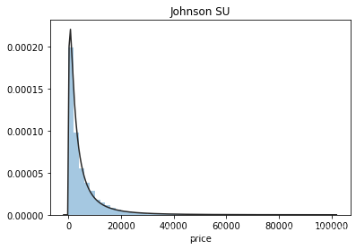
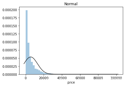

通过上面三幅图片,可以看出价格不服从正态分布,所以在进行回归之前,它必须进行转换。虽然对数变换做得很好,但最佳拟合是无界约翰逊分布
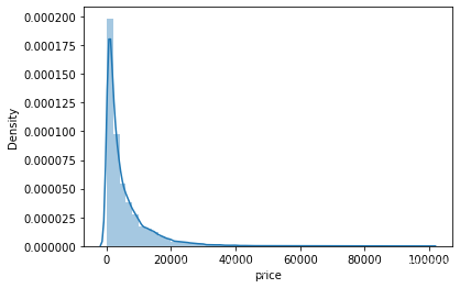
## 2) 查看skewness and kurtosis
sns.distplot(Train_data['price']);
print("Skewness: %f" % Train_data['price'].skew())
print("Kurtosis: %f" % Train_data['price'].kurt())
Skewness: 3.535346
Kurtosis: 21.230678
Train_data.skew(), Train_data.kurt()
(SaleID                0.001712
 name                  0.513079
 regDate              -1.540844
 model                 1.499765
 brand                 1.314846
 bodyType             -0.070459
 fuelType              0.701802
 gearbox              -1.357379
 power                58.590829
 kilometer            -1.557472
 notRepairedDamage    -2.312519
 regionCode            0.690405
 creatDate           -95.428563
 price                 3.535346
 v_0                  -1.504738
 v_1                   1.582428
 v_2                   1.198679
 v_3                   1.352193
 v_4                   0.217941
 v_5                   2.052749
 v_6                   0.090718
 v_7                   0.823610
 v_8                  -1.532964
 v_9                   1.529931
 v_10                 -2.584452
 v_11                 -0.906428
 v_12                 -2.842834
 v_13                 -3.869655
 v_14                  0.491706
 v_15                  1.308716
 v_16                  1.662893
 v_17                  0.233318
 v_18                  0.814453
 v_19                  0.100073
 v_20                  2.001253
 v_21                  0.180020
 v_22                  0.819133
 v_23                  1.357847
 dtype: float64,
 SaleID                  -1.201476
 name                    -1.084474
 regDate                 11.041006
 model                    1.741896
 brand                    1.814245
 bodyType                -1.070358
 fuelType                -1.495782
 gearbox                 -0.157525
 power                 4473.885260
 kilometer                1.250933
 notRepairedDamage        3.347777
 regionCode              -0.352973
 creatDate            11376.694263
 price                   21.230678
 v_0                      2.901641
 v_1                      1.098703
 v_2                      3.749872
 v_3                      4.294578
 v_4                      6.953348
 v_5                      6.489791
 v_6                     -0.564878
 v_7                     -0.729838
 v_8                      0.370812
 v_9                      0.377943
 v_10                     4.796855
 v_11                     1.547812
 v_12                     6.136342
 v_13                    13.199575
 v_14                    -1.597532
 v_15                    -0.029594
 v_16                     2.240928
 v_17                     2.569341
 v_18                     2.967738
 v_19                     6.923953
 v_20                     6.852809
 v_21                    -0.759948
 v_22                    -0.741708
 v_23                     0.143713
 dtype: float64)
通过上述偏度峰度的分析,creatData数据具有极不平衡的特性,通过它的分布密度图片来看,数据具有极不平衡的特性,有些信息效果不好
sns.distplot(Train_data['price']);

Train_data['creatDate'].value_counts()
20160403    9758
20160404    9521
20160320    9176
20160312    8946
20160321    8895
            ...
20150618       1
20160114       1
20160201       1
20150611       1
20140310       1
Name: creatDate, Length: 107, dtype: int64
sns.distplot(Train_data.skew(),color='blue',axlabel ='Skewness')

sns.distplot(Train_data.kurt(),color='orange',axlabel ='Kurtness')

## 3) 查看预测值的具体频数
plt.hist(Train_data['price'], orientation = 'vertical',histtype = 'bar', color ='red')
plt.show()

Train_data['price'] = np.maximum(Train_data['price'],0.1)
## log变换 z之后的分布较均匀,可以进行log变换进行预测,这也是预测问题常用的trick
plt.hist(np.log(Train_data['price']), orientation = 'vertical',histtype = 'bar', color ='red')
plt.show()

## 删除条件行的操作
Train_data1 = Train_data.drop(Train_data.index[Train_data['price'] <= 1])
## log变换 z之后的分布较均匀,可以进行log变换进行预测,这也是预测问题常用的trick
plt.hist(np.log(Train_data1['price']), orientation = 'vertical',histtype = 'bar', color ='red')
plt.show()

Train_data1.shape
(241897, 38)
通过这个频数图,可知已有的二手车训练集数据中售价超过两万的比例很低,因此这部分的信息价值并不高,预测的准确性会更差。
6.特征分为类别特征和数字特征,并对类别特征查看unique分布
# 分离label即预测值
Y_train = Train_data['price']
# 数字特征
numeric_features = Train_data.select_dtypes(include=[np.number])
numeric_features.columns
# # 类型特征
# categorical_features = Train_data.select_dtypes(include=[np.object])
# categorical_features.columns
categorical_features = ['name', 'model', 'brand', 'bodyType', 'fuelType', 'gearbox', 'notRepairedDamage', 'regionCode',]
# 特征nunique分布
for cat_fea in categorical_features:
    print(cat_fea + "的特征分布如下:")
    print("{}特征有个{}不同的值".format(cat_fea, Train_data[cat_fea].nunique()))
    print(Train_data[cat_fea].value_counts())
name的特征分布如下:
name特征有个164312不同的值
451       452
73        429
1791      428
821       391
243       346
         ...
92419       1
88325       1
82182       1
84231       1
157427      1
Name: name, Length: 164312, dtype: int64
model的特征分布如下:
model特征有个251不同的值
0.0      20344
6.0      17741
4.0      13837
1.0      13634
12.0      8841
         ...
226.0        5
245.0        5
243.0        4
249.0        4
250.0        1
Name: model, Length: 251, dtype: int64
brand的特征分布如下:
brand特征有个40不同的值
0     53699
4     27109
11    26944
10    23762
1     22144
6     17202
9     12210
5      7343
15     6500
12     4704
7      3839
3      3831
17     3543
13     3502
8      3374
28     3161
19     2561
18     2451
16     2274
22     2264
23     2088
14     1892
24     1678
25     1611
20     1610
27     1392
29     1259
34      963
30      604
2       570
31      540
21      522
38      516
35      415
32      406
36      377
33      368
37      324
26      307
39      141
Name: brand, dtype: int64
bodyType的特征分布如下:
bodyType特征有个8不同的值
7.0    64571
3.0    53858
4.0    45646
5.0    20343
6.0    15290
2.0    12755
1.0     9882
0.0     2275
Name: bodyType, dtype: int64
fuelType的特征分布如下:
fuelType特征有个7不同的值
0.0    150664
5.0     72494
4.0      3577
3.0       385
2.0       183
1.0       147
6.0        60
Name: fuelType, dtype: int64
gearbox的特征分布如下:
gearbox特征有个2不同的值
1.0    184645
0.0     51842
Name: gearbox, dtype: int64
notRepairedDamage的特征分布如下:
notRepairedDamage特征有个2不同的值
1.0    176922
0.0     24542
Name: notRepairedDamage, dtype: int64
regionCode的特征分布如下:
regionCode特征有个8081不同的值
487     550
868     424
149     236
539     227
32      216
       ...
7959      1
8002      1
6715      1
7117      1
4144      1
Name: regionCode, Length: 8081, dtype: int64
# 特征nunique分布
for cat_fea in categorical_features:
    print(cat_fea + "的特征分布如下:")
    print("{}特征有个{}不同的值".format(cat_fea, Test_data[cat_fea].nunique()))
    print(Test_data[cat_fea].value_counts())
name的特征分布如下:
name特征有个38668不同的值
73        98
821       89
243       77
451       74
826       73
          ..
106879     1
108926     1
176509     1
178556     1
67583      1
Name: name, Length: 38668, dtype: int64
model的特征分布如下:
model特征有个249不同的值
0.0      3916
6.0      3496
1.0      2806
4.0      2802
12.0     1745
         ...
247.0       2
246.0       2
214.0       1
243.0       1
232.0       1
Name: model, Length: 249, dtype: int64
brand的特征分布如下:
brand特征有个40不同的值
0     10697
4      5464
11     5374
10     4747
1      4390
6      3496
9      2408
5      1534
15     1325
12      929
7       782
3       736
17      732
13      679
8       666
28      645
19      534
18      487
16      458
22      430
14      416
23      397
24      390
25      297
20      293
27      265
29      236
34      206
30      133
21      121
2       101
38       92
31       87
35       76
36       73
26       72
32       70
37       61
33       61
39       40
Name: brand, dtype: int64
bodyType的特征分布如下:
bodyType特征有个8不同的值
7.0    12748
3.0    10808
4.0     9143
5.0     4175
6.0     3079
2.0     2484
1.0     1980
0.0      473
Name: bodyType, dtype: int64
fuelType的特征分布如下:
fuelType特征有个7不同的值
0.0    30045
5.0    14645
4.0      754
3.0       73
2.0       43
1.0       23
6.0       15
Name: fuelType, dtype: int64
gearbox的特征分布如下:
gearbox特征有个2不同的值
1.0    36935
0.0    10352
Name: gearbox, dtype: int64
notRepairedDamage的特征分布如下:
notRepairedDamage特征有个2不同的值
1.0    35555
0.0     4817
Name: notRepairedDamage, dtype: int64
regionCode的特征分布如下:
regionCode特征有个7078不同的值
487     122
868      93
539      46
32       46
222      46
       ...
3761      1
6232      1
7891      1
2106      1
2246      1
Name: regionCode, Length: 7078, dtype: int64
通过查看unique特征分布,可以对测试集与训练集数据分布情况进行比对
7.数字特征分析
相关性分析
查看几个特征得 偏度和峰值
每个数字特征得分布可视化
数字特征相互之间的关系可视化
多变量互相回归关系可视化
## 确定数据集中nan值的个数
Train_data1.isnull().sum()
SaleID                   0
name                     0
regDate                  0
model                    0
brand                    0
bodyType             22605
fuelType             19858
gearbox              11584
power                    0
kilometer                0
notRepairedDamage    44533
regionCode               0
creatDate                0
price                    0
v_0                      0
v_1                      0
v_2                      0
v_3                      0
v_4                      0
v_5                      0
v_6                      0
v_7                      0
v_8                      0
v_9                      0
v_10                     0
v_11                     0
v_12                     0
v_13                     0
v_14                     0
v_15                     0
v_16                     0
v_17                     0
v_18                     0
v_19                     0
v_20                     0
v_21                     0
v_22                     0
v_23                     0
dtype: int64
numeric_features = [col for col in numeric_features if col not in ['SaleID','name','bodyType','fuelType','gearbox','notRepairedDamage']]
numeric_features
['regDate',
 'model',
 'brand',
 'power',
 'kilometer',
 'regionCode',
 'creatDate',
 'price',
 'v_0',
 'v_1',
 'v_2',
 'v_3',
 'v_4',
 'v_5',
 'v_6',
 'v_7',
 'v_8',
 'v_9',
 'v_10',
 'v_11',
 'v_12',
 'v_13',
 'v_14',
 'v_15',
 'v_16',
 'v_17',
 'v_18',
 'v_19',
 'v_20',
 'v_21',
 'v_22',
 'v_23']
## 1) 相关性分析
price_numeric = Train_data1[numeric_features]
correlation = price_numeric.corr()
print(correlation['price'].sort_values(ascending = False),'\n')
price         1.000000
v_0           0.521790
v_11          0.499157
v_15          0.414843
regDate       0.313313
power         0.193045
v_8           0.171495
v_10          0.153313
v_22          0.148351
v_7           0.148020
model         0.144848
v_12          0.116560
v_13          0.103143
v_14          0.064229
v_19          0.036949
v_20          0.030306
regionCode    0.016943
v_4           0.011313
creatDate    -0.003412
v_2          -0.008591
brand        -0.010469
v_23         -0.018257
v_5          -0.025231
v_6          -0.043621
v_21         -0.055471
v_17         -0.102734
v_9          -0.150717
v_1          -0.189762
v_16         -0.332209
kilometer    -0.420236
v_18         -0.597190
v_3          -0.679661
Name: price, dtype: float64
f , ax = plt.subplots(figsize = (7, 7))

plt.title('Correlation of Numeric Features with Price',y=1,size=16)

sns.heatmap(correlation,square = True,  vmax=0.8)

del price_numeric['price']
## 2) 查看几个特征得 偏度和峰值
for col in numeric_features:
    print('{:15}'.format(col),
          'Skewness: {:05.2f}'.format(Train_data[col].skew()) ,
          '   ' ,
          'Kurtosis: {:06.2f}'.format(Train_data[col].kurt())
         )
regDate         Skewness: -1.54     Kurtosis: 011.04
model           Skewness: 01.50     Kurtosis: 001.74
brand           Skewness: 01.31     Kurtosis: 001.81
power           Skewness: 58.59     Kurtosis: 4473.89
kilometer       Skewness: -1.56     Kurtosis: 001.25
regionCode      Skewness: 00.69     Kurtosis: -00.35
creatDate       Skewness: -95.43     Kurtosis: 11376.69
price           Skewness: 03.54     Kurtosis: 021.23
v_0             Skewness: -1.50     Kurtosis: 002.90
v_1             Skewness: 01.58     Kurtosis: 001.10
v_2             Skewness: 01.20     Kurtosis: 003.75
v_3             Skewness: 01.35     Kurtosis: 004.29
v_4             Skewness: 00.22     Kurtosis: 006.95
v_5             Skewness: 02.05     Kurtosis: 006.49
v_6             Skewness: 00.09     Kurtosis: -00.56
v_7             Skewness: 00.82     Kurtosis: -00.73
v_8             Skewness: -1.53     Kurtosis: 000.37
v_9             Skewness: 01.53     Kurtosis: 000.38
v_10            Skewness: -2.58     Kurtosis: 004.80
v_11            Skewness: -0.91     Kurtosis: 001.55
v_12            Skewness: -2.84     Kurtosis: 006.14
v_13            Skewness: -3.87     Kurtosis: 013.20
v_14            Skewness: 00.49     Kurtosis: -01.60
v_15            Skewness: 01.31     Kurtosis: -00.03
v_16            Skewness: 01.66     Kurtosis: 002.24
v_17            Skewness: 00.23     Kurtosis: 002.57
v_18            Skewness: 00.81     Kurtosis: 002.97
v_19            Skewness: 00.10     Kurtosis: 006.92
v_20            Skewness: 02.00     Kurtosis: 006.85
v_21            Skewness: 00.18     Kurtosis: -00.76
v_22            Skewness: 00.82     Kurtosis: -00.74
v_23            Skewness: 01.36     Kurtosis: 000.14
## 3) 每个数字特征得分布可视化
f = pd.melt(Train_data1, value_vars=numeric_features)
g = sns.FacetGrid(f, col="variable",  col_wrap=2, sharex=False, sharey=False)
g = g.map(sns.distplot, "value")

Train_data1.head()
| SaleID | name | regDate | model | brand | bodyType | fuelType | gearbox | power | kilometer | ... | v_14 | v_15 | v_16 | v_17 | v_18 | v_19 | v_20 | v_21 | v_22 | v_23 | |
|---|---|---|---|---|---|---|---|---|---|---|---|---|---|---|---|---|---|---|---|---|---|
| 0 | 134890 | 734 | 20160002 | 13.0 | 9 | NaN | 0.0 | 1.0 | 0 | 15.0 | ... | 0.092139 | 0.000000 | 18.763832 | -1.512063 | -1.008718 | -12.100623 | -0.947052 | 9.077297 | 0.581214 | 3.945923 |
| 1 | 306648 | 196973 | 20080307 | 72.0 | 9 | 7.0 | 5.0 | 1.0 | 173 | 15.0 | ... | 0.001070 | 0.122335 | -5.685612 | -0.489963 | -2.223693 | -0.226865 | -0.658246 | -3.949621 | 4.593618 | -1.145653 |
| 2 | 340675 | 25347 | 20020312 | 18.0 | 12 | 3.0 | 0.0 | 1.0 | 50 | 12.5 | ... | 0.064410 | 0.003345 | -3.295700 | 1.816499 | 3.554439 | -0.683675 | 0.971495 | 2.625318 | -0.851922 | -1.246135 |
| 3 | 57332 | 5382 | 20000611 | 38.0 | 8 | 7.0 | 0.0 | 1.0 | 54 | 15.0 | ... | 0.069231 | 0.000000 | -3.405521 | 1.497826 | 4.782636 | 0.039101 | 1.227646 | 3.040629 | -0.801854 | -1.251894 |
| 4 | 265235 | 173174 | 20030109 | 87.0 | 0 | 5.0 | 5.0 | 1.0 | 131 | 3.0 | ... | 0.000099 | 0.001655 | -4.475429 | 0.124138 | 1.364567 | -0.319848 | -1.131568 | -3.303424 | -1.998466 | -1.279368 |
5 rows × 38 columns
## 4) 数字特征相互之间的关系可视化
sns.set()
columns = ['price', 'v_12', 'v_8' , 'v_0', 'power', 'v_5',  'v_2', 'v_6', 'v_1', 'v_14']
sns.pairplot(Train_data1[columns],size = 2 ,kind ='scatter',diag_kind='kde')
plt.show()

## 5) 多变量互相回归关系可视化
fig, ((ax1, ax2), (ax3, ax4), (ax5, ax6), (ax7, ax8), (ax9, ax10)) = plt.subplots(nrows=5, ncols=2, figsize=(24, 20))
# ['v_12', 'v_8' , 'v_0', 'power', 'v_5',  'v_2', 'v_6', 'v_1', 'v_14']
v_12_scatter_plot = pd.concat([Y_train,Train_data1['v_12']],axis = 1)
sns.regplot(x='v_12',y = 'price', data = v_12_scatter_plot,scatter= True, fit_reg=True, ax=ax1)

v_8_scatter_plot = pd.concat([Y_train,Train_data1['v_8']],axis = 1)
sns.regplot(x='v_8',y = 'price',data = v_8_scatter_plot,scatter= True, fit_reg=True, ax=ax2)

v_0_scatter_plot = pd.concat([Y_train,Train_data1['v_0']],axis = 1)
sns.regplot(x='v_0',y = 'price',data = v_0_scatter_plot,scatter= True, fit_reg=True, ax=ax3)

power_scatter_plot = pd.concat([Y_train,Train_data1['power']],axis = 1)
sns.regplot(x='power',y = 'price',data = power_scatter_plot,scatter= True, fit_reg=True, ax=ax4)

v_5_scatter_plot = pd.concat([Y_train,Train_data1['v_5']],axis = 1)
sns.regplot(x='v_5',y = 'price',data = v_5_scatter_plot,scatter= True, fit_reg=True, ax=ax5)

v_2_scatter_plot = pd.concat([Y_train,Train_data1['v_2']],axis = 1)
sns.regplot(x='v_2',y = 'price',data = v_2_scatter_plot,scatter= True, fit_reg=True, ax=ax6)

v_6_scatter_plot = pd.concat([Y_train,Train_data1['v_6']],axis = 1)
sns.regplot(x='v_6',y = 'price',data = v_6_scatter_plot,scatter= True, fit_reg=True, ax=ax7)

v_1_scatter_plot = pd.concat([Y_train,Train_data1['v_1']],axis = 1)
sns.regplot(x='v_1',y = 'price',data = v_1_scatter_plot,scatter= True, fit_reg=True, ax=ax8)

v_14_scatter_plot = pd.concat([Y_train,Train_data1['v_14']],axis = 1)
sns.regplot(x='v_14',y = 'price',data = v_14_scatter_plot,scatter= True, fit_reg=True, ax=ax9)

v_13_scatter_plot = pd.concat([Y_train,Train_data1['v_13']],axis = 1)
sns.regplot(x='v_13',y = 'price',data = v_13_scatter_plot,scatter= True, fit_reg=True, ax=ax10)

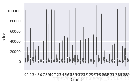
8.类型特征分析
unique分布
类别特征箱形图可视化
类别特征的小提琴图可视化
类别特征的柱形图可视化类别
特征的每个类别频数可视化(count_plot)
## 1) unique分布
for fea in categorical_features:
    print(Train_data1[fea].nunique())
250
40
8
7
2
2
categorical_features
['model', 'brand', 'bodyType', 'fuelType', 'gearbox', 'notRepairedDamage']
## 2) 类别特征箱形图可视化

# 因为 name和 regionCode的类别太稀疏了,这里我们把不稀疏的几类画一下
categorical_features = ['model',
 'brand',
 'bodyType',
 'fuelType',
 'gearbox',
 'notRepairedDamage']
for c in categorical_features:
    Train_data1[c] = Train_data1[c].astype('category')
    if Train_data1[c].isnull().any():
        Train_data1[c] = Train_data1[c].cat.add_categories(['MISSING'])
        Train_data1[c] = Train_data1[c].fillna('MISSING')

def boxplot(x, y, **kwargs):
    sns.boxplot(x=x, y=y)
    x=plt.xticks(rotation=90)

f = pd.melt(Train_data1, id_vars=['price'], value_vars=categorical_features)
g = sns.FacetGrid(f, col="variable",  col_wrap=2, sharex=False, sharey=False, size=5)
g = g.map(boxplot, "value", "price")

## 3) 类别特征的小提琴图可视化
catg_list = categorical_features
target = 'price'
for catg in catg_list :
    sns.violinplot(x=catg, y=target, data=Train_data)
    plt.show()

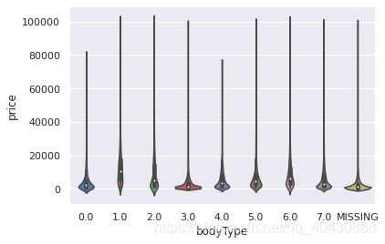
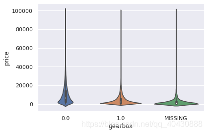
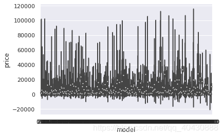
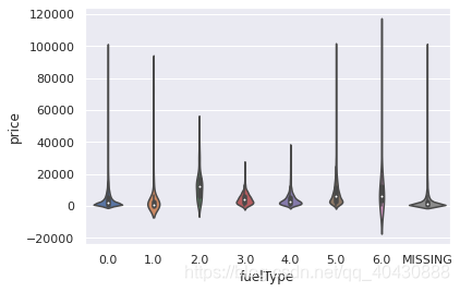
[外链图片转存失败,源站可能有防盗链机制,建议将图片保存下来直接上传(img-zHNJrHWh-1618539021565)(output_70_0.png)]
categorical_features = ['model',
 'brand',
 'bodyType',
 'fuelType',
 'gearbox',
 'notRepairedDamage']
## 4) 类别特征的柱形图可视化
def bar_plot(x, y, **kwargs):
    sns.barplot(x=x, y=y)
    x=plt.xticks(rotation=90)

f = pd.melt(Train_data, id_vars=['price'], value_vars=categorical_features)
g = sns.FacetGrid(f, col="variable",  col_wrap=2, sharex=False, sharey=False, size=5)
g = g.map(bar_plot, "value", "price")

##  5) 类别特征的每个类别频数可视化(count_plot)
def count_plot(x,  **kwargs):
    sns.countplot(x=x)
    x=plt.xticks(rotation=90)

f = pd.melt(Train_data,  value_vars=categorical_features)
g = sns.FacetGrid(f, col="variable",  col_wrap=2, sharex=False, sharey=False, size=5)
g = g.map(count_plot, "value")

9.用pandas_profiling生成数据报告
用pandas_profiling生成一个较为全面的可视化和数据报告(较为简单、方便) 最终打开html文件即可
import pandas_profiling
pfr = pandas_profiling.ProfileReport(Train_data)
pfr.to_file("./example.html")
第一遍可惜崩溃了,所以单独写了个文件跑界面,html界面也卡顿,应该是数据太大的缘故,这个建议报告可以取一些变量分批生成报告,生成的报告在资源里


 被折叠的 条评论
为什么被折叠?
被折叠的 条评论
为什么被折叠?
 到【灌水乐园】发言


