WRF后处理| 画图时的投影

说在前面：

本来想整理一下WRF后处理中风向图、风羽图的相关代码，途中忽然注意到了WRF投影的问题，因此进行了相关资料整理和探讨。根据WRF用户手册：

As a general guideline, the polar stereographic proiection is best suited for high-latitude WRF domains, the Lambert conformal projection is well-suited for mid-latitude domains, and the Mercator projection is good for low-latitude domains or domains with predominantly west-east extent. The cylindrical equidistant projection is required for global ARW simulations, although in its rotated aspect (i.e.,when pole_lat, pole_lon, and stand_lon are changed from their default values) it can also be well-suited for regional domains anywhere on the earth’s surface.
------------------------------------------------------《WRF-ARW V3: User’s Guide》

也就是说，极地投影最适合高纬度，大约60°以上；兰伯特投影最适合中纬度，大约30°-60°；而墨卡托投影最适合低纬度，大约30°S-30°N或以东西向为主的区域。等距圆柱投影适合全球的模拟，它可以很好地适用于地球表面任何地方的区域。但其实WRF的使用中，一般使用的都是兰伯特投影，用户手册中的案例也多次使用兰伯特投影。

不同投影的画图是怎么样的：

兰伯特：

import matplotlib.pyplot as plt
import cartopy.crs as ccrs
import netCDF4 as nc
from cartopy.mpl.gridliner import LONGITUDE_FORMATTER, LATITUDE_FORMATTER
from wrf import (to_np, getvar, get_cartopy, latlon_coords)
import cartopy.crs as crs
import numpy as np

data = nc.Dataset('G:\WRF/wrfout_d01_2023-04-08_00_00_00')
slp = getvar(data, "T2")
lats, lons = latlon_coords(slp)
cart_proj = get_cartopy(slp)
fig = plt.figure(figsize=(12,6))
ax = plt.axes(projection=cart_proj)
plt.contour(to_np(lons), to_np(lats), to_np(slp), colors="black",
            transform=crs.PlateCarree())
mesh=plt.contourf(to_np(lons), to_np(lats), to_np(slp), 
              transform=crs.PlateCarree())
colorbar=plt.colorbar(ax=ax, shrink=.98)
mesh = ax.gridlines(draw_labels=True, linestyle='--', linewidth=0.6, alpha=0.5, x_inline=False, y_inline=False, color='k')
mesh.top_labels=False
mesh.right_labels=False
mesh.xformatter = LONGITUDE_FORMATTER
mesh.yformatter = LATITUDE_FORMATTER
ax.set_extent([113,115.5,21.5,23.5],crs=ccrs.PlateCarree()) 

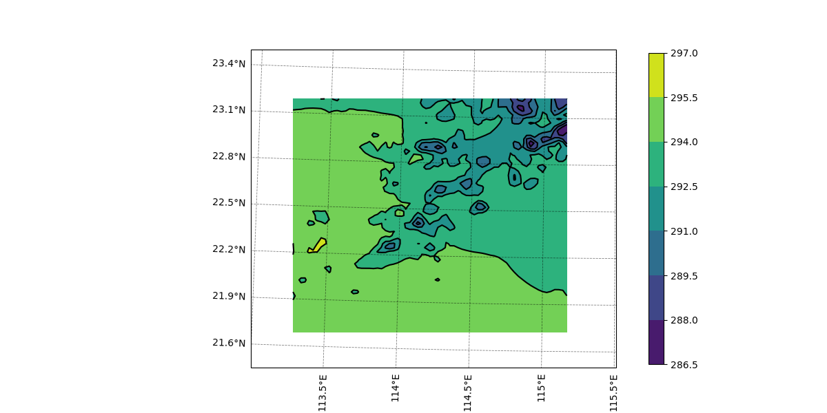
圆柱投影：

import matplotlib.pyplot as plt
import cartopy.crs as ccrs
import netCDF4 as nc
from cartopy.mpl.gridliner import LONGITUDE_FORMATTER, LATITUDE_FORMATTER
from wrf import (to_np, getvar, get_cartopy, latlon_coords)
import cartopy.crs as crs
import numpy as np
# In[]
data = nc.Dataset('G:\WRF/wrfout_d01_2023-04-08_00_00_00')
slp = getvar(data, "T2")
lats, lons = latlon_coords(slp)
fig = plt.figure(figsize=(12, 6))
ax = fig.add_subplot(111, projection=ccrs.PlateCarree())
  
plt.contour(to_np(lons), to_np(lats), to_np(slp), colors="black",
            transform=crs.PlateCarree())
mesh=plt.contourf(to_np(lons), to_np(lats), to_np(slp), 
              transform=crs.PlateCarree())
colorbar=plt.colorbar(ax=ax, shrink=.98)
mesh = ax.gridlines(draw_labels=True, linestyle='--', linewidth=0.6, alpha=0.5, x_inline=False, y_inline=False, color='k')
mesh.top_labels=False
mesh.right_labels=False
mesh.xformatter = LONGITUDE_FORMATTER
mesh.yformatter = LATITUDE_FORMATTER
ax.set_extent([113,115.5,21.5,23.5],crs=ccrs.PlateCarree()) # 小范围

两个图的区别其实很明显，一个是经纬度网格斜了，一个是色斑块斜了。由于WRF模拟时选择的投影方式是兰伯特投影，所以当画图时依然采用兰伯特投影时，他就是一个正正方方的网格。但放在圆柱投影这种等经纬度投影时，由于投影的不同，画出来的图就是斜的。
我们习惯使用的是等经纬度投影画图，对于没有方向性的标量画图，画出来的图无非就是斜的，问题不大。但如果具有方向性的话，比如风场，就需要进行风向的调整，因为采用兰伯特投影的WRF输出数据，风场的东南西北是沿着经纬度网格的，它的经纬度网格并不是我们传统意义平面上的上下左右，而是斜的，所以需要进行风向的调整，但是该点的风速大小不变。
WRF最常用的模型有兰伯特投影，极地投影和墨卡托投影。对于墨卡托投影，不需要风向的调整，对于兰伯特投影和极地投影，需要风向的调整。关于风向代码的整理被耽误了，下一篇再发吧。