连续LTI系统的时域响应

连续LTI系统的时域响应

① 求零状态响应的MATLAB程序



卷积结果：
yt =2t - heaviside(t - 1)(2t - 2) - heaviside(t - 2)(2t - 4) + heaviside(t - 3)(2*t - 6)


3、已知描述系统的微分方程和激励信号e(t) 分别如下

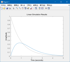
试用解析方法求系统的单位冲激响应h(t)和零状态响应r(t)，并用MATLAB绘出系统单位冲激响应和系统零状态响应的波形，验证结果是否相同。
① 求冲激响应的MATLAB程序


② 求零状态响应的MATLAB程序

三、
%求冲激响应的MATLAB程序：
a=[1 4 4];
b=[1 3];
subplot(2,1,1), impulse(b,a,4)


%求零状态响应的MATLAB程序方法1：
a=[1 4 4];
b=[1  3];
p1=0.001;    %定义取样时间间隔为0.001
t1=0:p1:5;     %定义时间范围
x1=exp(-1*t1).*heaviside(t1);    %定义输入信号
lsim(b,a,x1,t1),     %对取样间隔为0.001时系统响应进行仿真
%求零状态响应的MATLAB程序方法1：
a=[1 4 4];
b=[0 1 3];
p1=0.001;    %定义取样时间间隔为0.001
t1=0:p1:5;     %定义时间范围
x1=exp(-1*t1).*heaviside(t1);    %定义输入信号
lsim(b,a,x1,t1),     %对取样间隔为0.001时系统响应进行仿真


%零状态响应方法2
eq1='Dy+4*Dy+4*y=Dx+3*x';
eq2='x=exp(-1*t)*heaviside(t)';
cond='y(-0.001)=0,Dy(-0.001)=0';
yzs=dsolve(eq1,eq2,cond);
yzs=simplify(yzs.y);
ezplot(yzs,[0,8]);grid on
title('零状态响应');
%零状态响应方法2
eq1='Dy+4*Dy+4*y=Dx+3*x';
eq2='x=exp(-1*t).*heaviside(t)';
cond='y(-0.01)=0,Dy(-0.01)=0';
yzs=dsolve(eq1,eq2,cond);
yzs=simplify(yzs.y);
ezplot(yzs,[0,5]);grid on
title('零状态响应');
******************************************************************

二、
%方法一
t0 = -4; t1 = 4; dt = 0.01;
t = t0:dt:t1;
x = 2*(heaviside(t+1)-heaviside(t-1));
h = heaviside(t+2)-heaviside(t-2);
y = dt*conv(x,h); % Compute the convolution of x(t) and h(t)
subplot(221)
plot(t,x), grid on, title('Signal x(t)'), axis([t0,t1,-0.2,2])
subplot(222)
plot(t,h), grid on, title('Signal h(t)'), axis([t0,t1,-0.2,2])
subplot(212)
t = 2*t0:dt:2*t1; % Again specify the time range to be suitable to the
% convolution of x and h.
plot(t,y), grid on, title('The convolution of x(t) and h(t)'),
axis([2*t0,2*t1,-0.1,6]),
xlabel('Time t sec')

方法三
p=0.01;
k1=-4:p:4;
f1=2*(heaviside(k1+1)-heaviside(k1-1));
k2=-4:p:4;
f2=heaviside(k2+2)-heaviside(k2-2);
[f,k]=sconv(f1,f2,k1,k2,p)
************************************************************************四、
%零输入响应：
eq='D2y+4*Dy+4*y=0';
cond='y(0)=0,Dy(0)=1';
yzi=dsolve(eq,cond);
yzi=simplify(yzi);
%零状态响应： 
eq1='D2y+4*Dy+4*y=Dx+3*x';
eq2='x=exp(-1*t)*heaviside(t)';
cond='y(-0.001)=0,Dy(-0.001)=0';
yzs=dsolve(eq1,eq2,cond);
yzs=simplify(yzs.y);
yt=simplify(yzi+yzs);

subplot(311)
ezplot(yzi,[0,8]);grid on
title('零输入响应');
subplot(312)
ezplot(yzs,[0,8]);grid on
title('零状态响应');
subplot(313)
ezplot(yt,[0,8]);grid on
title('全响应');

五、
t0 = -2; t1 = 4; dt = 0.01;
t = t0:dt:t1;
x = heaviside(t)-heaviside(t-1);
h = t.*(heaviside(t)-heaviside(t-1));
y = dt*conv(x,h); % Compute the convolution of x(t) and h(t)
subplot(221)
plot(t,x), grid on, title('Signal x(t)'), axis([t0,t1,-0.2,1.2])
subplot(222)
plot(t,h), grid on, title('Signal h(t)'), axis([t0,t1,-0.2,1.2])
subplot(212)
t = 2*t0:dt:2*t1; % Again specify the time range to be suitable to the
% convolution of x and h.
plot(t,y), grid on, title('The convolution of x(t) and h(t)'),
axis([2*t0,2*t1,-0.1,0.6]),
xlabel('Time t sec')
*****************************************************
t0 = -2; t1 = 4; dt = 0.1;
t = t0:dt:t1;
x = heaviside(t)-heaviside(t-1);
h = t.*(heaviside(t)-heaviside(t-1));
y = dt*conv(x,h); % Compute the convolution of x(t) and h(t)
subplot(221)
plot(t,x), grid on, title('Signal x(t)'), axis([t0,t1,-0.2,1.2])
subplot(222)
plot(t,h), grid on, title('Signal h(t)'), axis([t0,t1,-0.2,1.2])
subplot(212)
t = 2*t0:dt:2*t1; % Again specify the time range to be suitable to the
% convolution of x and h.
plot(t,y), grid on, title('The convolution of x(t) and h(t)'),
axis([2*t0,2*t1,-0.1,0.6]),
xlabel('Time t sec')

*****************************
t0 = -2; t1 = 4; dt = 1;
t = t0:dt:t1;
x = heaviside(t)-heaviside(t-1);
h = t.*(heaviside(t)-heaviside(t-1));
y = dt*conv(x,h); % Compute the convolution of x(t) and h(t)
subplot(221)
plot(t,x), grid on, title('Signal x(t)'), axis([t0,t1,-0.2,1.2])
subplot(222)
plot(t,h), grid on, title('Signal h(t)'), axis([t0,t1,-0.2,1.2])
subplot(212)
t = 2*t0:dt:2*t1; % Again specify the time range to be suitable to the
% convolution of x and h.
plot(t,y), grid on, title('The convolution of x(t) and h(t)'),
axis([2*t0,2*t1,-0.1,0.6]),
xlabel('Time t sec')
*********************************
t0 = -2; t1 = 4; dt = 0.001;
t = t0:dt:t1;
x = heaviside(t)-heaviside(t-1);
h = t.*(heaviside(t)-heaviside(t-1));
y = dt*conv(x,h); % Compute the convolution of x(t) and h(t)
subplot(221)
plot(t,x), grid on, title('Signal x(t)'), axis([t0,t1,-0.2,1.2])
subplot(222)
plot(t,h), grid on, title('Signal h(t)'), axis([t0,t1,-0.2,1.2])
subplot(212)
t = 2*t0:dt:2*t1; % Again specify the time range to be suitable to the
% convolution of x and h.
plot(t,y), grid on, title('The convolution of x(t) and h(t)'),
axis([2*t0,2*t1,-0.1,0.6]),
xlabel('Time t sec')