opencv-python笔记（一）

入门：opencv-python-code

图像基础

读入显示图像

import cv2
import numpy as np
from matplotlib import pyplot as plt

img = cv2.imread('img/1.jpg',0)
cv2.imshow('image',img) 
#cv2.namedWindow('image', cv2.WINDOW_NORMAL) #在新窗口中显示

用matplotlib 显示图像

plt.imshow(img, cmap='gray', interpolation='bicubic')
#camp='gray'表示显示灰度图像，若默认则为RGB模式，但是OpenCV读取为BGR模式所以会有问题
plt.xticks([]), plt.yticks([])
plt.show()

按键退出

## 键入esc时退出，s保存退出
k = cv2.waitKey(0)
if k == 27:
   cv2.destoryAllWindows()
elif k == ord('s'):
   cv2.immwrite('img/1.jpg', img)
   cv2.destoryAllWindows()

视频基础

视频操作

# 打开摄像头并灰度化显示
import cv2
capture = cv2.VideoCapture(0)
# 播放本地视频 capture = cv2.VideoCapture('demo_video.mp4')
while(True):
    # 获取一帧
    ret, frame = capture.read()
    # 将这帧转换为灰度图
    gray = cv2.cvtColor(frame, cv2.COLOR_BGR2GRAY)
    cv2.imshow('frame', gray)
    if cv2.waitKey(1) == ord('q'):
        break

录制视频

capture = cv2.VideoCapture(0)
# 定义编码方式并创建VideoWriter对象
fourcc = cv2.VideoWriter_fourcc(*'MJPG')
outfile = cv2.VideoWriter('output.avi', fourcc, 25., (640, 480))
while(capture.isOpened()):
    ret, frame = capture.read()
    if ret:
        outfile.write(frame)  # 写入文件
        cv2.imshow('frame', frame)
        if cv2.waitKey(1) == ord('q'):
            break
    else:
        break

图像基本操作

获取像素点

import cv2

img = cv2.imread('demo.png')
px = img[100,90]
print(px) 
#结果是 bgr三个值
px_blue = img[100, 90, 0]
print(px_blue)
#结果对比

图片属性

print(img.shape)  # (263, 247, 3)
# 形状中包括行数、列数和通道数
height, width, channels = img.shape
# img是灰度图的话：height, width = img.shape
print(img.dtype)  # uint8
print(img.size)  # 263*247*3=194883

ROI

# 截取ROI
face = img[100:200, 115:188]
cv2.imshow('face', face)
cv2.waitKey(0)

通道的分割与合并

cv2.split()拆分通道&&&cv2.merge()合并通道

b, g, r = cv2.split(img)
img = cv2.merge((b, g, r))

推荐利用numpy高效地提取通道

b = img[:, :, 0]
cv2.imshow('blue', b)
cv2.waitKey(0)

阈值分割

cv2.threshold()&&&cv2.adaptiveThreshold

cv2.threshold()用来实现阈值分割，ret是return value缩写，代表当前的阈值，暂时不用理会。函数有4个参数：

• 参数1：要处理的原图，一般是灰度图
• 参数2：设定的阈值
• 参数3：最大阈值，一般为255
• 参数4：阈值的方式，主要有5种，详情：ThresholdTypes
  EX:

    import matplotlib.pyplot as plt
    # 应用5种不同的阈值方法
    ret, th1 = cv2.threshold(img, 127, 255, cv2.THRESH_BINARY)
    ret, th2 = cv2.threshold(img, 127, 255, cv2.THRESH_BINARY_INV)
    ret, th3 = cv2.threshold(img, 127, 255, cv2.THRESH_TRUNC)
    ret, th4 = cv2.threshold(img, 127, 255, cv2.THRESH_TOZERO)
    ret, th5 = cv2.threshold(img, 127, 255, cv2.THRESH_TOZERO_INV)
    titles = ['Original', 'BINARY', 'BINARY_INV', 'TRUNC', 'TOZERO', 'TOZERO_INV']
    images = [img, th1, th2, th3, th4, th5]
    # 使用Matplotlib显示
    for i in range(6):
        plt.subplot(2, 3, i + 1)
        plt.imshow(images[i], 'gray')
        plt.title(titles[i], fontsize=8)
        plt.xticks([]), plt.yticks([])  # 隐藏坐标轴
    plt.show()

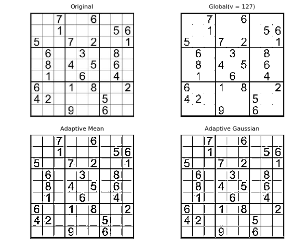
自适应阈值分割

看得出来固定阈值是在整幅图片上应用一个阈值进行分割，它并不适用于明暗分布不均的图片。 cv2.adaptiveThreshold()自适应阈值会每次取图片的一小部分计算阈值，这样图片不同区域的阈值就不尽相同。它有5个参数，其实很好理解，先看下效果：

# 自适应阈值对比固定阈值
img = cv2.imread('sudu.jpg', 0)
# 固定阈值
ret, th1 = cv2.threshold(img, 127, 255, cv2.THRESH_BINARY)
# 自适应阈值

th2 = cv2.adaptiveThreshold(
    img, 255, cv2.ADAPTIVE_THRESH_MEAN_C, cv2.THRESH_BINARY, 11, 4)
th3 = cv2.adaptiveThreshold(
    img, 255, cv2.ADAPTIVE_THRESH_GAUSSIAN_C, cv2.THRESH_BINARY, 17, 6)
titles = ['Original', 'Global(v = 127)', 'Adaptive Mean', 'Adaptive Gaussian']
images = [img, th1, th2, th3]
for i in range(4):
    plt.subplot(2, 2, i + 1), plt.imshow(images[i], 'gray')
    plt.title(titles[i], fontsize=8)
    plt.xticks([]), plt.yticks([])
plt.show()

自适应阈值对比固定阈值

OTSU算法

Otsu算法假设这副图片由前景色和背景色组成，通过统计学方法（最大类间方差）选取一个阈值，将前景和背景尽可能分开，我们先来看下代码，然后详细说明下算法原理。

import cv2
from matplotlib import pyplot as plt
img = cv2.imread('noisy.jpg', 0)
# 固定阈值法
ret1, th1 = cv2.threshold(img, 100, 255, cv2.THRESH_BINARY)
# Otsu阈值法
ret2, th2 = cv2.threshold(img, 0, 255, cv2.THRESH_BINARY + cv2.THRESH_OTSU)
# 先进行高斯滤波，再使用Otsu阈值法
blur = cv2.GaussianBlur(img, (5, 5), 0)
ret3, th3 = cv2.threshold(blur, 0, 255, cv2.THRESH_BINARY + cv2.THRESH_OTSU)


images = [img, 0, th1, img, 0, th2, blur, 0, th3]
titles = ['Original', 'Histogram', 'Global(v=100)',
          'Original', 'Histogram', "Otsu's",
          'Gaussian filtered Image', 'Histogram', "Otsu's"]
for i in range(3):
    # 绘制原图
    plt.subplot(3, 3, i * 3 + 1)
    plt.imshow(images[i * 3], 'gray')
    plt.title(titles[i * 3], fontsize=8)
    plt.xticks([]), plt.yticks([])
    # 绘制直方图plt.hist，ravel函数将数组降成一维
    plt.subplot(3, 3, i * 3 + 2)
    plt.hist(images[i * 3].ravel(), 256)
    plt.title(titles[i * 3 + 1], fontsize=8)
    plt.xticks([]), plt.yticks([])
    # 绘制阈值图
    plt.subplot(3, 3, i * 3 + 3)
    plt.imshow(images[i * 3 + 2], 'gray')
    plt.title(titles[i * 3 + 2], fontsize=8)
    plt.xticks([]), plt.yticks([])
plt.show()

OTSU算法降噪阈值分割

图像几何变换

缩放

cv2.resize()

import cv2
img = cv2.imread('drawing.jpg')
# 按照指定的宽度、高度缩放图片
res = cv2.resize(img, (132, 150))
# 按照比例缩放，如x,y轴均放大一倍
res2 = cv2.resize(img, None, fx=2, fy=2, interpolation=cv2.INTER_LINEAR)
cv2.imshow('shrink', res), cv2.imshow('zoom', res2)
cv2.waitKey(0)

翻转

cv2.flip()

import cv2
img = cv2.imread('demo.jpg')
dst = cv2.flip(img, 1)
cv2.imshow('flipped', img)
cv2.waitKey(0)
#其中，参数2 = 0：垂直翻转(沿x轴)，参数2 > 0: 水平翻转(沿y轴)，参数2 < 0: 水平垂直翻转。

平移

cv2.warpAffine()

import cv2
import numpy as np
img = cv2.imread('demo.jpg')
rows, cols = img.shape[:2]
# 定义平移矩阵，需要是numpy的float32类型
# x轴平移100，y轴平移50
M = np.float32([[1, 0, 100], [0, 1, 50]])
# 用仿射变换实现平移
dst = cv2.warpAffine(img, M, (cols, rows))
cv2.imshow('shift', dst)
cv2.waitKey(0)

旋转

旋转同平移一样，也是用仿射变换实现的，因此也需要定义一个变换矩阵。OpenCV直接提供了 cv2.getRotationMatrix2D()函数来生成这个矩阵，该函数有三个参数：

• 参数1：图片的旋转中心
• 参数2：旋转角度(正：逆时针，负：顺时针)
• 参数3：缩放比例，0.5表示缩小一半

import cv2
import numpy as np
img = cv2.imread('demo.jpg')
rows, cols = img.shape[:2]
# 定义平移矩阵，需要是numpy的float32类型
# x轴平移100，y轴平移50
M = np.float32([[1, 0, 100], [0, 1, 50]])
# 用仿射变换实现平移
M = cv2.getRotationMatrix2D((cols / 2, rows / 2), 45, 0.5)
dst = cv2.warpAffine(img, M, (cols, rows))
cv2.imshow('rotation', dst)
cv2.waitKey(0)

仿射变换

import cv2
import numpy as np
import matplotlib.pyplot as plt
img = cv2.imread('noisy.jpg')
rows, cols = img.shape[:2]
# 变换前的三个点
pts1 = np.float32([[50, 65], [150, 65], [210, 210]])
# 变换后的三个点
pts2 = np.float32([[50, 100], [150, 65], [100, 250]])
# 生成变换矩阵
M = cv2.getAffineTransform(pts1, pts2)
dst = cv2.warpAffine(img, M, (cols, rows))
plt.subplot(121), plt.imshow(img), plt.title('input')
plt.subplot(122), plt.imshow(dst), plt.title('output')
plt.show()

变换	矩阵	自由度	保持性质
平移	[I, t]	（2×3）	2
刚体	[R, t]	（2×3）	3
相似	[sR, t]	（2×3）	4
仿射	[T]	（2×3）	6
透视	[T]	（3×3）	8

透视变换

透视变换是将二维的图片投影到一个三维视平面上，然后再转换到二维坐标下，所以也称为投影映射（Projective Mapping）。简单来说就是二维→三维→二维的一个过程。
透视变换相比仿射变换更加灵活，变换后会产生一个新的四边形，但不一定是平行四边形，所以需要非共线的四个点才能唯一确定，原图中的直线变换后依然是直线。因为四边形包括了所有的平行四边形，所以透视变换包括了所有的仿射变换。
OpenCV中首先根据变换前后的四个点用cv2.getPerspectiveTransform()生成3×3的变换矩阵，然后再用cv2.warpPerspective()进行透视变换。实战演练一下

img = cv2.imread('card.jpg')
# 原图中卡片的四个角点
pts1 = np.float32([[61, 71], [162, 30], [151, 217], [270, 145]])
# 变换后分别在左上、右上、左下、右下四个点
pts2 = np.float32([[0, 0], [320, 0], [0, 450], [320, 450]])
# 生成透视变换矩阵
M = cv2.getPerspectiveTransform(pts1, pts2)
# 进行透视变换，参数3是目标图像大小
dst = cv2.warpPerspective(img, M, (320, 450))
plt.subplot(121), plt.imshow(img[:, :, ::-1]), plt.title('input')
plt.subplot(122), plt.imshow(dst[:, :, ::-1]), plt.title('output')
plt.show()
# matplotlib 读图RGB模式，openCV BGR模式 需要-1的参数调整

poker示例

绘图功能

画线

# 创建一副黑色的图片
img = np.zeros((512, 512, 3), np.uint8)
# 画一条线宽为5的蓝色直线，参数2：起点，参数3：终点
cv2.line(img, (0, 0), (512, 512), (255, 0, 0), 5)

画矩形

画矩形需要知道左上角和右下角的坐标：

# 画一个绿色边框的矩形，参数2：左上角坐标，参数3：右下角坐标
cv2.rectangle(img, (384, 0), (510, 128), (0, 255, 0), 3)

画圆

画圆需要指定圆心和半径，注意下面的例子中线宽=-1代表填充：

# 画一个填充红色的圆，参数2：圆心坐标，参数3：半径
cv2.circle(img, (447, 63), 63, (0, 0, 255), -1)

画椭圆

画椭圆需要的参数比较多，请对照后面的代码理解这几个参数：

参数2：椭圆中心(x,y)
参数3：x/y轴的长度
参数4：angle—椭圆的旋转角度
参数5：startAngle—椭圆的起始角度
参数6：endAngle—椭圆的结束角度
经验之谈：OpenCV中原点在左上角，所以这里的角度是以顺时针方向计算的。

# 在图中心画一个填充的半圆
cv2.ellipse(img, (256, 256), (100, 50), 0, 0, 180, (255, 0, 0), -1)

画多边形

画多边形需要指定一系列多边形的顶点坐标，相当于从第一个点到第二个点画直线，再从第二个点到第三个点画直线….

OpenCV中需要先将多边形的顶点坐标需要变成顶点数×1×2维的矩阵，再来绘制：

# 定义四个顶点坐标
pts = np.array([[10, 5],  [50, 10], [70, 20], [20, 30]], np.int32)
# 顶点个数：4，矩阵变成4*1*2维
pts = pts.reshape((-1, 1, 2))
cv2.polylines(img, [pts], True, (0, 255, 255))
cv2.polylines()的参数3如果是False的话，多边形就不闭合。

经验之谈：如果需要绘制多条直线，使用cv2.polylines()要比cv2.line()高效很多，例如：

# 使用cv2.polylines()画多条直线
line1 = np.array([[100, 20],  [300, 20]], np.int32).reshape((-1, 1, 2))
line2 = np.array([[100, 60],  [300, 60]], np.int32).reshape((-1, 1, 2))
line3 = np.array([[100, 100],  [300, 100]], np.int32).reshape((-1, 1, 2))
cv2.polylines(img, [line1, line2, line3], True, (0, 255, 255))

添加文字

使用cv2.putText()添加文字，它的参数也比较多，同样请对照后面的代码理解这几个参数：

参数2：要添加的文本
参数3：文字的起始坐标（左下角为起点）
参数4：字体
参数5：文字大小（缩放比例）

# 添加文字
font = cv2.FONT_HERSHEY_SIMPLEX
cv2.putText(img, 'ex2tron', (10, 500), font,
            4, (255, 255, 255), 2, lineType=cv2.LINE_AA)

完整示例

import cv2
import numpy as np

# 创建一副黑色的图片
img = np.zeros((512, 512, 3), np.uint8)
# 1.画一条线宽为5的蓝色直线，参数2：起点，参数3：终点
cv2.line(img, (0, 0), (512, 512), (255, 0, 0), 5)


# 2.画一个绿色边框的矩形，参数2：左上角坐标，参数3：右下角坐标
cv2.rectangle(img, (384, 0), (510, 128), (0, 255, 0), 3)


# 3.画一个填充红色的圆，参数2：圆心坐标，参数3：半径
cv2.circle(img, (447, 63), 63, (0, 0, 255), -1)


# 4.在图中心画一个填充的半圆
cv2.ellipse(img, (256, 256), (100, 50), 0, 0, 180, (255, 0, 0), -1)


# 5.画一个闭合的四边形
# 定义四个顶点坐标
pts = np.array([[10, 5],  [50, 10], [70, 20], [20, 30]], np.int32)
# 顶点个数：4，矩阵变成顶点数*1*2维（注意numpy中-1的用法）
pts = pts.reshape((-1, 1, 2))
cv2.polylines(img, [pts], True, (0, 255, 255))

# 使用cv2.polylines()画多条直线
line1 = np.array([[100, 20],  [300, 20]], np.int32).reshape((-1, 1, 2))
line2 = np.array([[100, 60],  [300, 60]], np.int32).reshape((-1, 1, 2))
line3 = np.array([[100, 100],  [300, 100]], np.int32).reshape((-1, 1, 2))
cv2.polylines(img, [line1, line2, line3], True, (0, 255, 255))


# 6.添加文字
font = cv2.FONT_HERSHEY_SIMPLEX
cv2.putText(img, 'COOLSYN', (10, 500), font,
            4, (255, 255, 255), 2, lineType=cv2.LINE_AA)

cv2.imshow('img', img)
cv2.waitKey(0)`

画图样式

鼠标画图

import cv2
import numpy as np
drawing = False  # 是否开始画图
mode = True  # True：画矩形，False：画圆
start = (-1, -1)
def mouse_event(event, x, y, flags, param):
    global start, drawing, mode
    # 左键按下：开始画图
    if event == cv2.EVENT_LBUTTONDOWN:
        drawing = True
        start = (x, y)
    # 鼠标移动，画图
    elif event == cv2.EVENT_MOUSEMOVE:
        if drawing:
            if mode:
                cv2.rectangle(img, start, (x, y), (0, 255, 0), 1)
            else:
                cv2.circle(img, (x, y), 5, (0, 0, 255), -1)
    # 左键释放：结束画图
    elif event == cv2.EVENT_LBUTTONUP:
        drawing = False
        if mode:
            cv2.rectangle(img, start, (x, y), (0, 255, 0), 1)
        else:
            cv2.circle(img, (x, y), 5, (0, 0, 255), -1)
img = np.zeros((512, 512, 3), np.uint8)
cv2.namedWindow('image')
cv2.setMouseCallback('image', mouse_event)
while(True):
    cv2.imshow('image', img)
    # 按下m切换模式
    if cv2.waitKey(1) == ord('m'):
        mode = not mode
    elif cv2.waitKey(1) == 27:
        break

效果图