%% ========== 子函数9: comparePercentileFilteringWithLOF ==========
function [filtered_original, filtered_after_lof, lofOutlierMask, x_seg, y_seg] = ...
comparePercentileFilteringWithLOF(rawData, varargin)
% comparePercentileFilteringWithLOF_Optimized - 对比两种滤波策略:
%
% 方法1: 原始信号 → 百分位滤波
% 方法2: LOF去异常 + 插值 → 百分位滤波
%
% 输入:
% rawData - Nx1 或 Nx2 数值矩阵
% 名值对参数:
% 'TargetLength' - 截取长度,默认 5000
% 'Percentile' - 百分位数,默认 5
% 'WindowLength' - 滑动窗口长度,默认 101
% 'ShowPlot' - 是否绘图,默认 true
%
% 输出:
% filtered_original - 方法一的滤波结果
% filtered_after_lof - 方法二的滤波结果
% lofOutlierMask - 异常点逻辑数组
% x_seg - 时间索引(截取段)
% y_seg - 原始熔深值(截取段)
%% 参数解析
%该部分定义并解析一组可输入参数,用于控制信号或数据预处理行为,常用于数据清洗,异常检测,平滑处理等场景
p = inputParser;
addOptional(p, 'TargetLength', 5000, @isnumeric);
addOptional(p, 'Percentile', 5, @(x) isnumeric(x) && x >= 0 && x <= 100);
addOptional(p, 'WindowLength', 101, @(x) isnumeric(x) && mod(x,2)==1 && x >= 3);
addOptional(p, 'ShowPlot', true, @islogical);
parse(p, varargin{:});
targetNum = p.Results.TargetLength;
pct_value = p.Results.Percentile;
windowLen = p.Results.WindowLength;
showPlot = p.Results.ShowPlot;
%% 输入验证
if isempty(rawData)
warning('⚠️ 无法执行对比分析:输入数据为空!');
filtered_original = []; filtered_after_lof = []; lofOutlierMask = [];
x_seg = []; y_seg = [];
return;
end
if ~isnumeric(rawData) || ~ismatrix(rawData)
error('❌ rawData 必须是数值矩阵。');
end
% 提取 y
if size(rawData, 2) >= 2
y_full = rawData(:, 2);
else
y_full = rawData(:);
end
x_full = (1:length(y_full))';
nTotal = length(y_full);
if nTotal < 3
error('❌ 数据点太少,无法进行分析(至少需要3个点)。');
end
%% 截取中间段
idxStart = 1; idxEnd = nTotal;
if nTotal > targetNum
mid = floor(nTotal / 2);
half = floor(targetNum / 2);
idxStart = max(1, mid - half + 1);
idxEnd = min(nTotal, mid + half);
end
% 确保 x_seg 和 y_seg 是同长度列向量
x_seg = (idxStart:idxEnd)'; % 列向量
y_seg = y_full(idxStart:idxEnd); % 提取子集
y_seg = y_seg(:); % 强制列向量
n = length(y_seg);
fprintf('🔍 开始对比分析:处理区间 [%d, %d],样本数=%d\n', idxStart, idxEnd, n);
if n < 3
error('❌ 截取后数据少于3个点,无法进行分析。');
end
%% 步骤1:使用优化版 LOF 检测异常点(复用已有函数)
try
[~, isOutlier, ~, ~] = performLOFOnWDP_Optimized([x_seg, y_seg], ...
'TargetLength', targetNum, ...
'KFactor', 0.01, ...
'UseMedianIQR', true, ...
'ShowPlot', false);
catch ME
warningId = 'WDPAnalysis:LOF:ExecutionFailed';
warning(warningId, 'LOF 异常检测执行失败:%s。将跳过去噪步骤并使用原始信号进行滤波。', ME.message);
isOutlier = false(n, 1); % 默认无异常点
end
numOutliers = sum(isOutlier);
lofOutlierMask = isOutlier;
fprintf('📊 LOF检测完成,发现 %d 个异常点\n', numOutliers);
%% 步骤2:构建两组输入信号
% --- 方法一:原始完整信号 ---
y_original = y_seg;
% --- 方法二:去除异常点后插值补全 ---
y_clean = y_seg;
y_clean(isOutlier) = NaN;
% 使用 pchip 插值(保形,减少振荡)
y_interpolated = interp1(x_seg(~isOutlier), y_clean(~isOutlier), x_seg, 'pchip');
% 边界处理:若首尾为NaN,则用最近邻填充
if any(isnan(y_interpolated))
missingIdx = isnan(y_interpolated);
y_interpolated(missingIdx) = interp1(x_seg(~missingIdx), y_interpolated(~missingIdx), ...
x_seg(missingIdx), 'nearest');
end
%% 步骤3:分别执行滑动百分位滤波(调用优化函数)
filtered_original = slidingPercentileFilter(y_original, windowLen, pct_value);
filtered_after_lof = slidingPercentileFilter(y_interpolated, windowLen, pct_value);
%% 步骤4:绘制双子图对比
if showPlot
fig = figure('Position', [100, 100, 800, 600], ...
'Name', '【对比】百分位滤波 vs LOF+百分位滤波', ...
'Color', 'white');
set(fig, 'DefaultAxesFontName', 'Microsoft YaHei');
set(fig, 'DefaultTextFontName', 'Microsoft YaHei');
set(fig, 'GraphicsSmoothing', 'on');
% 子图1:原始 → 百分位滤波
subplot(2,1,1);
hold on;
plot(x_seg, y_original, 'Color', [0.7 0.7 0.7], 'LineWidth', 0.8, 'DisplayName', '原始实测点');
plot(x_seg, filtered_original, 'k-', 'LineWidth', 1.8, 'DisplayName', sprintf('%g%% 滤波', pct_value));
title(sprintf('方法一:直接对原始数据进行 %g%% 百分位滤波', pct_value));
legend('show', 'Location', 'bestoutside');
grid on; box on; hold off;
ylabel('熔深值 (mm)');
% 子图2:LOF去噪后 → 百分位滤波
subplot(2,1,2);
hold on;
plot(x_seg, y_interpolated, 'Color', [0.9 0.9 0.9], 'LineWidth', 0.8, 'DisplayName', 'LOF去噪+插值');
plot(x_seg, filtered_after_lof, 'b-', 'LineWidth', 1.8, 'DisplayName', ['LOF+' sprintf('%g%%滤波', pct_value)]);
scatter(x_seg(isOutlier), y_seg(isOutlier), 30, 'r', 'filled', ...
'DisplayName', sprintf('LOF异常点(n=%d)', numOutliers), 'MarkerFaceAlpha', 0.8);
title(sprintf('方法二:先LOF去噪再进行 %g%% 百分位滤波', pct_value));
legend('show', 'Location', 'bestoutside');
grid on; box on; hold off;
xlabel('时间索引');
ylabel('熔深值 (mm)');
sgtitle({'💡 LOF预处理提升滤波稳定性'; ...
sprintf('窗口=%d, 百分位=%g%%, 异常点=%d/%d', windowLen, pct_value, numOutliers, n)}, ...
'FontSize', 12, 'FontWeight', 'bold');
drawnow;
end
disp('✅ 双子图对比已完成:显示了是否使用LOF预处理的影响。');
end
%% ========== 子函数 2: findTargetFiles ==========
function targetFiles = findTargetFiles(folderPath, extensions, keywords)
% 查找每个关键词对应的首个匹配文件(按扩展名遍历)
%
% 输入:
% folderPath - 目标文件夹路径(字符串)
% extensions - 扩展名通配符元胞数组,如 {'*.csv', '*.txt', '*.dat'}
% keywords - 关键词元胞数组,如 {'WD','WDP','WDS','WDSQ'}
% 输出:
% targetFiles - 元胞数组,每个元素对应找到的第一个匹配文件的完整路径;
% 未找到则为空字符串 ''
% cell就是用于创建一个空的元胞数据,这就相当于把关键词元胞数组的尺寸给复制下来
targetFiles = cell(size(keywords));
fprintf('🔍 正在搜索目录:%s\n', folderPath);
for i = 1:length(keywords)
%这里found就只是一个真假逻辑的引出值,用于后续判断
found = false;
fprintf('🔍 开始查找关键词 "%s"...\n', keywords{i});
for e = 1:length(extensions)
extName = extensions{e};
searchPattern = fullfile(folderPath, extName);
files = dir(searchPattern);
fprintf(' → 检查 %s: 共发现 %d 个文件\n', extName, length(files));
for k = 1:length(files)
filename = files(k).name;
if contains(filename, keywords{i}, 'IgnoreCase', true)
targetFiles{i} = fullfile(folderPath, filename);
fprintf('✅ 匹配第%d个文件: %s (来自 %s)\n', i, filename, extName);
found = true;
break;
end
end
if found, break; end
end
if ~found
warning('⚠️ 未找到包含 "%s" 的文件!', keywords{i});
targetFiles{i} = '';
end
end
%% ========== 子函数 7-1: getFilterParamsFromDialog ==========
% 局部函数:getFilterParamsFromDialog
% 必须放在文件末尾!
% ===========================================================================
function [p_val, w_len] = getFilterParamsFromDialog(p_default, w_default)
%prompt就是一个引导用户输入的函数
prompt = {'请输入百分位数 (建议 0-10):', '请输入滑动窗口长度 (推荐奇数):'};
dlgTitle = '📊 百分位滤波参数设置';
defaults = {p_default, w_default};
%等价于条件成立时,执行后边的语句,否则结束
if isempty(defaults{1}), defaults{1} = '5'; end
if isempty(defaults{2}), defaults{2} = '101'; end
%inputdlg函数:弹出一个模态对话框,提示用户输入参数,并将用户的输入以字符串元胞数组的形式返回
answer = inputdlg(prompt, dlgTitle, 1, defaults);
if isempty(answer)
p_val = [];
w_len = [];
else
p_val = str2double(answer{1});
w_len = str2double(answer{2});
if isnan(p_val)
error('❌ 百分位输入无效,请输入合法数字!');
end
if isnan(w_len)
error('❌ 窗口长度输入无效,请输入整数!');
end
end
end
%% ========== 子函数 8: performLOFOnWDP_Optimized ==========
function [lofScores, isOutlier, x_sub, y_sub] = performLOFOnWDP_Optimized(rawData, varargin)
% performLOFOnWDP_Optimized - 基于 y 和变化率的 LOF 异常检测(向量化加速 + 多阈值策略)
%
% 输入:
% rawData - Nx1 或 Nx2 数值矩阵,列2为熔深值
% 名值对参数:
% 'TargetLength' - 截取长度,默认 5000
% 'UseMedianIQR' - 是否使用中位数 IQR 抗噪,默认 true
% 'KFactor' - k = floor(n * KFactor),默认 0.01
% 'ShowPlot' - 是否绘图,默认 true
%
% 输出:
% lofScores - 每个样本的 LOF 得分
% isOutlier - 逻辑数组,标记是否为异常点
% x_sub - 时间索引(截取后)
% y_sub - 熔深值(截取后)
%% 参数解析
%给定一个inputParser变量
p = inputParser;
addOptional(p, 'TargetLength', 5000, @(x) isnumeric(x) && isscalar(x) && x > 0);
addOptional(p, 'UseMedianIQR', true, @islogical);
addOptional(p, 'KFactor', 0.01, @(x) isnumeric(x) && x > 0 && x <= 0.1);
addOptional(p, 'ShowPlot', true, @islogical);
parse(p, varargin{:});
targetNum = p.Results.TargetLength;
useMedianIQR = p.Results.UseMedianIQR;
kFactor = p.Results.KFactor;
showPlot = p.Results.ShowPlot;
%% 输入验证
if isempty(rawData)
warning('⚠️ 输入数据为空!');
lofScores = []; isOutlier = []; x_sub = []; y_sub = [];
return;
end
%ismatrix用于判断是不是一个二维数值矩阵
if ~isnumeric(rawData) || ~ismatrix(rawData)
error('❌ rawData 必须是数值矩阵。');
end
% 提取 y 列
if size(rawData, 2) >= 2
y = rawData(:, 2); % 第二列为熔深
else
y = rawData(:); % 单列直接使用
end
nTotal = length(y);
if nTotal < 3
error('❌ 数据点太少,无法进行 LOF 分析(至少需要3个点)。');
end
%% 截取中间段(用于大信号降复杂度)
idxStart = 1;
idxEnd = nTotal;
if nTotal > targetNum
mid = floor(nTotal / 2);
half = floor(targetNum / 2);
idxStart = max(1, mid - half + 1);
idxEnd = min(nTotal, mid + half);
end
x_sub = (idxStart:idxEnd)'; % 时间索引(列向量)
y_sub = y(idxStart:idxEnd); % 对应熔深值(列向量)
n = length(y_sub);
fprintf('📊 执行 LOF 分析:处理区间 [%d, %d],样本数=%d\n', idxStart, idxEnd, n);
%% 特征工程:[熔深值, 一阶差分, 二阶差分]
%diff就是相邻的前后作差分
dy = diff([y_sub; y_sub(end)]); % 补全最后一个 dy
ddy = diff([dy; dy(end)]); % 补全 ddy
features = [y_sub, dy, ddy]; % Nx3 特征矩阵
%% 归一化:Z-score 标准化
%mean可以对单列数,也可以对指定的数组列/行直接进行取平均值操作
mu = mean(features, 1);
sigma = std(features, 0, 1);
sigma(sigma == 0) = 1; % 防止除零
%./matlab用于逐个元素进行除法的操作
data_norm = (features - mu) ./ sigma;
%% 自适应 k 值选择
k = min(20, max(3, floor(kFactor * n)));
fprintf('🔍 使用 k = %d 进行 LOF 计算(样本数=%d)...\n', k, n);
%% 向量化计算欧氏距离矩阵
D = pdist2(data_norm, data_norm); % n×n 距离矩阵
%% 获取 k-近邻索引(排除自身)
%sort是对数组进行排序的内置函数
[~, sortedIdx] = sort(D, 2);
kNN_idx = sortedIdx(:, 2:k+1); % 每行前 k 个最近邻
%% 计算可达距离 reachDist(i,j) = max(d(i,j), rk_distance(j))
%repmat((1:n)', 1, k)将列向量横向复制k次,行程一个n*k的矩阵
%sub2ind用于将二维下标转换为线性索引,以便从矩阵中直接提取元素
r_k_dist = D(sub2ind(size(D), repmat((1:n)', 1, k), kNN_idx));
reachDistMat = zeros(n, k);
for i = 1:n
for j_idx = 1:k
j = kNN_idx(i, j_idx);
reachDistMat(i, j_idx) = max(D(i, j), r_k_dist(j, j_idx));
end
end
% 平均可达距离
avgReachDist = mean(reachDistMat, 2);
%% 局部可达密度 LRD = 1 / avgReachDist
LRD = 1 ./ (avgReachDist + eps);
%% LOF 得分:LOF(i) = mean(LRD of kNN(i)) / LRD(i)
lofScores = zeros(n, 1);
for i = 1:n
neighbor_LRDs = LRD(kNN_idx(i, :));
lofScores(i) = mean(neighbor_LRDs) / LRD(i);
end
%% 自适应阈值判定
Q1 = prctile(lofScores, 25);
Q3 = prctile(lofScores, 75);
IQR = Q3 - Q1;
if useMedianIQR
%median用于进行中位数的计算
threshold = median(lofScores) + 3 * IQR; % 更鲁棒
else
threshold = Q3 + 1.5 * IQR; % 经典方法
end
isOutlier = lofScores > threshold;
%sum就是进行异常点个数的统计
numOutliers = sum(isOutlier);
fprintf('✅ LOF 分析完成:共发现 %d 个异常点(阈值=%.3f)\n', numOutliers, threshold);
%% 可视化
if showPlot
fig = figure('Position', [400, 400, 800, 500], ...
'Name', '【优化版】LOF 异常检测结果', ...
'Color', 'white');
set(fig, 'DefaultAxesFontName', 'Microsoft YaHei');
set(fig, 'DefaultTextFontName', 'Microsoft YaHei');
set(fig, 'GraphicsSmoothing', 'on');
hold on; grid on; box on;
% 正常点
plot(x_sub(~isOutlier), y_sub(~isOutlier), 'b.', 'MarkerSize', 4, ...
'DisplayName', '正常点');
% 异常点
plot(x_sub(isOutlier), y_sub(isOutlier), 'ro', 'MarkerSize', 8, ...
'MarkerFaceColor', 'none', 'LineWidth', 2, ...
'DisplayName', sprintf('异常点(n=%d)', numOutliers));
xlabel('时间索引');
ylabel('熔深值 (mm)');
title(sprintf('LOF 异常检测结果\nk=%d, 阈值=%.3f, 异常占比=%.1f%%', ...
k, threshold, 100*numOutliers/n));
legend('show', 'Location', 'bestoutside');
hold off;
drawnow;
end
%% 输出统计信息
disp(['📈 LOF得分范围: ', num2str(min(lofScores), '%.5f'), ' ~ ', num2str(max(lofScores), '%.5f')]);
if numOutliers == 0
warning('🟡 未发现明显异常点,请检查信号是否过于平稳或需降低灵敏度');
end
end
%% ========== 子函数 7: performPercentileFiltering ==========
function [filteredY, x] = performPercentileFiltering(rawData, varargin)
% performPercentileFiltering - 对 WDP 数据进行百分位滤波并可视化
%
% 输入:
% rawData - Nx1 或 Nx2 数值矩阵
% 名值对参数:
% 'Percentile' - 百分位数 (0~100),默认弹窗输入
% 'WindowLength' - 滑动窗口长度(奇数),默认弹窗输入
% 'ShowPlot' - 是否绘图,true/false,默认 true
%
% 输出:
% filteredY - 滤波后的 y 序列
% x - 对应的时间/索引序列
%% 默认参数解析
%创建一个inputParser对象,后续所有参数都添加到这个对象中进行管理
p = inputParser;
%addOptional给对象p添加可选位置参数
addOptional(p, 'Percentile', [], @isnumeric);
%这里对名称(名称对应的位置),名称的类型都作了规定,下面几条语句也是的
addOptional(p, 'WindowLength', [], @isnumeric);
%silogical表明传入的一定要是逻辑型
addOptional(p, 'ShowPlot', true, @islogical);
%将变长输入参数varargin拆开并传给parse函数,inputParser会自动按顺序匹配这些参数到前面定义的addOptional列表中
%执行验证,失败则抛出错误,成功后可通过p.Results获取结果
parse(p, varargin{:});
%将通过inputParser成功解析的输入参数,从p.Results结构体中取出并幅值给局部变量
showPlot = p.Results.ShowPlot;
percentileValue = p.Results.Percentile;
windowLength = p.Results.WindowLength;
%% 输入验证
if isempty(rawData)
warning('⚠️ 无法进行滤波:输入数据为空!');
if showPlot
figure('Name', '滤波提示', 'Color', 'w');
text(0.5, 0.5, '无数据可处理', 'HorizontalAlignment', 'center', ...
'FontSize', 14, 'Color', 'r', 'FontWeight', 'bold');
title('百分位滤波失败');
end
filteredY = [];
x = [];
return;
end
if ~isnumeric(rawData) || ~ismatrix(rawData)
error('❌ rawData 必须是数值矩阵。');
end
% 提取 x 和 y
if size(rawData, 2) >= 2
x = rawData(:, 1);
y = rawData(:, 2);
else
x = (1:length(rawData))';
y = rawData(:);
end
n = length(y);
if n < 3
error('❌ 数据点太少,无法应用滑动窗口滤波(至少需要3个点)。');
end
%% 参数获取方式:优先名值对,否则弹窗
if isempty(percentileValue) || isempty(windowLength)
[p_val, w_len] = getFilterParamsFromDialog(percentileValue, windowLength);
if nargin == 1 && (isempty(p_val) || isempty(w_len))
warning('跳过滤波:用户取消输入。');
filteredY = y;
return;
end
percentileValue = p_val;
windowLength = w_len;
end
% 参数校验
if percentileValue < 0 || percentileValue > 100
error('❌ 百分位必须在 0~100 范围内!');
end
%isscalar是用于判断是不是标量的,mod函数则可以用于判断输入量的第一位小数是不是0,以此判断是不是整数
if windowLength < 3 || ~isscalar(windowLength) || mod(windowLength,1) ~= 0
error('❌ 窗口长度必须是大于等于3的整数!');
end
if mod(windowLength, 2) == 0
warning('⚠️ 窗口长度应为奇数,已自动调整为 %d', windowLength + 1);
windowLength = windowLength + 1;
end
%% 执行滑动窗口百分位滤波(镜像边界扩展)
%floor就是用于向下取整
halfWin = floor(windowLength / 2);
%下面这个是将整体拼接为一个向量,前向镜像填充+原始数据+后向镜像填充
%函数flipud就是进行列向量的上下翻转,fliplr就是进行行向量的上下翻转
y_ext = [flipud(y(1:halfWin)); y; flipud(y(end-halfWin+1:end))];
filteredY = zeros(n, 1);
for i = halfWin + 1 : n + halfWin
windowData = y_ext(i - halfWin : i + halfWin);
%prctile用于计算百分数,最终返回第输入百分位
filteredY(i - halfWin) = prctile(windowData, percentileValue);
end
%% 可视化
if showPlot
fig = figure('Position', [300, 300, 800, 500], ...
'Name', sprintf('%g%% 百分位滤波结果', percentileValue), ...
'Color', 'white');
set(fig, 'DefaultAxesFontName', 'Microsoft YaHei');
set(fig, 'DefaultTextFontName', 'Microsoft YaHei');
set(fig, 'GraphicsSmoothing', 'on');
hold on; grid on;
scatter(x, y, 6, [0.5 0.5 1], 'filled', ...
'MarkerFaceAlpha', 0.5, 'DisplayName', '原始实测点');
plot(x, filteredY, 'Color', [1, 0, 0], 'LineWidth', 2, ...
'DisplayName', sprintf('%g%% 百分位滤波曲线', percentileValue));
xlabel('时间 / 索引');
ylabel('熔深值 (mm)');
title(sprintf('WDP 数据滤波结果(窗口=%d, 百分位=%.1f%%)', windowLength, percentileValue));
legend('show', 'Location', 'best', 'Box', 'off');
box on;
drawnow;
end
% 日志输出
fprintf('🔧 已完成 %.1f%% 百分位滤波处理,窗口大小=%d,数据长度=%d\n', ...
percentileValue, windowLength, n);
end
%% ========== 子函数 3: readDataSafely ==========
function data = readDataSafely(filePath)
% readDataSafely - 安全读取数值型表格数据(支持 CSV/TXT/DAT/XLSX)
% 输入:
% filePath - 文件路径(字符串)
% 输出:
% data - 数值型矩阵(double),MxN
%
% 特性:
% - 自动检测分隔符和编码
% - 支持多种格式(包括 Excel)
% - 优先使用现代函数(readmatrix)
% - 兜底策略清晰
% - 提供详细错误信息
%% 输入验证
if nargin < 1 || isempty(filePath) || ~ischar(filePath)
error('❌ 输入参数 filePath 必须是非空字符串。');
end
if ~isfile(filePath)
error('❌ 指定的文件不存在:%s', filePath);
end
fprintf('📊 正在读取数据文件: %s\n', filePath);
%% 第一尝试:使用 readmatrix(推荐方式)
try
% 兼容旧版本写法
%detectImoportOptions内置函数:分析指定文本文件的内容结构,并生成一个导入选项对象
opts = detectImportOptions(filePath);
%readmatrix内置函数:用于读取纯数值矩阵数据的函数
data = readmatrix(filePath, opts); % 自动处理分隔符、标题行等
%isnumeric判断数据是否为数值类型
if isnumeric(data) && ~isempty(data)
fprintf('✅ 成功使用 readmatrix 读取数据,尺寸: %d×%d\n', size(data));
return;
else
warning('⚠️ readmatrix 返回了空或非数值数据,尝试备用方法...');
end
catch ME1
fprintf('💡 readmatrix 失败: %s\n', ME1.message);
end
%% 第二尝试:readtable + 转换(兼容复杂表结构)
try
opts = detectImportOptions(filePath);
%对读取的文件的命名进行规范,保留原始列名
opts.VariableNamingRule = 'preserve';
%readtable函数:读取为表格结构/类型
tbl = readtable(filePath, opts);
% 检查所有变量是否可转为数值
%这里也是相当于引出一个变量作为逻辑值的载体,表示某种含义与否
allNumeric = true;
%width函数:输入的列数的读取
for i = 1:width(tbl)
%tb1{:,i};提取第i列的所有行,并尝试将其内容转换为一个数值向量或字符数组
var = tbl{:,i};
%any()函数:判断至少是否至少含有某一个指定量
if ~isnumeric(var) || any(isnan(var)) % 注意:字符转数字失败会引入 NaN
allNumeric = false;
break;
end
end
if allNumeric
%table2array函数:将表格类型变量转换为普通的数值数组
data = table2array(tbl);
fprintf('✅ 成功用 readtable 读取并转换为数值矩阵,尺寸: %d×%d\n', size(data));
return;
else
warning('⚠️ 表格中包含非数值列,跳过 readtable 方法...');
end
catch ME2
fprintf('💡 readtable 失败: %s\n', ME2.message);
end
%% 第三尝试:旧式 csvread(仅限 .csv 文件且纯数字)
try
%fileparts函数:分解文件路径字符串的内置函数,分解为路径、名字、类型
[~, ~, ext] = fileparts(filePath);
%strcmpi函数:2个字符串是否相等,且不区分类型的大小写
if strcmpi(ext, '.csv')
%csvread函数:从指定的CSV文件路径中读取纯数值数据
data = csvread(filePath);
if isnumeric(data) && ~isempty(data)
fprintf('✅ 成功用 csvread 读取数据(兼容模式),尺寸: %d×%d\n', size(data));
return;
end
end
catch ME3
fprintf('💡 csvread 失败: %s\n', ME3.message);
end
%% 所有方法均失败
error('❌ 所有读取方法均失败,无法加载文件:\n%s', filePath);
%% ========== 子函数 1: selectFolder ==========
function folderPath = selectFolder(defaultPath)
%% 参数处理与默认值
%判断输入参数个数,或者输入是否为空或者非字符串类型
if nargin < 1 || isempty(defaultPath) || ~ischar(defaultPath)
%pwd是内置函数,用于使用当前工作目录为默认路径,确保程序有可用的起点
defaultPath = pwd;
%isfolder是函数,用于检查指定路径是否存在,并且判断是不是一个文件夹
elseif ~isfolder(defaultPath)
warning('⚠️ 指定的默认路径不存在,将使用当前工作目录:\n%s', defaultPath);
defaultPath = pwd;
end
fprintf('🔍 正在打开文件夹选择器,默认路径: %s\n', defaultPath);
titleStr = '请选择焊接数据所在文件夹';
%uigetdir内置函数:打开一个图形化的选择文件夹对话框,允许鼠标点击浏览并选择目录
folderPath = uigetdir(defaultPath, titleStr);
if folderPath == 0
error('❌ 用户取消了文件夹选择,程序终止。');
end
% 规范化路径分隔符
%strrep就是将原路径下的符号更改为指定符号
folderPath = strrep(folderPath, '\', '/');
fprintf('✅ 已选择工作目录: %s\n', folderPath);
end
%% ========== 子函数9—1: slidingPercentileFilter ==========
function result = slidingPercentileFilter(signal, windowLen, pct)
% slidingPercentileFilter_Vec - 向量化滑动窗口百分位滤波
%
% 输入:
% signal - 一维信号
% windowLen - 奇数窗口长度
% pct - 百分位数 (0~100)
%
% 输出:
% result - 滤波后信号
n = length(signal);
result = zeros(n, 1);
halfWin = floor(windowLen / 2);
% 边界保持原样
result(1:halfWin) = signal(1:halfWin);
result(end-halfWin+1:end) = signal(end-halfWin+1:end);
% 中心区域:使用 movprctile 思路(若无工具箱则手动向量化)
%exist函数:检查类型文件是否存在
if exist('movprctile', 'file') % Statistics and Machine Learning Toolbox
result(halfWin+1:n-halfWin) = movprctile(signal, pct, windowLen);
else
% 手动构造滑动窗口(利用 arrayfun 向量化)
idx_center = (halfWin + 1):(n - halfWin);
windows = arrayfun(@(i) signal(i-halfWin : i+halfWin), idx_center, 'UniformOutput', false);
result(halfWin+1:n-halfWin) = cellfun(@(w) prctile(w, pct), windows);
end
end
%% ========== 子函数 4: subsampleData ==========
function result = subsampleData(data, step)
% subsampleData - 通用降采样函数(支持多种模式)
% 输入:
% data - 二维数值矩阵(MxN),每行为一个样本
% step - 正整数,采样间隔;即每 step 行取一行
% 输出:
% result - 降采样后的矩阵(KxN),K ≈ ceil(M/step)
%% 输入验证
if nargin < 2
error('❌ 缺少必要输入参数:需要 data 和 step。');
end
if isempty(data)
fprintf('🔍 输入数据为空,返回空矩阵。\n');
result = [];
return;
end
if ~isnumeric(data) || ~ismatrix(data)
error('❌ data 必须是非空二维数值矩阵。');
end
if ~isscalar(step) || ~isnumeric(step) || step <= 0 || floor(step) ~= step
error('❌ step 必须是正整数。');
end
%size函数:读取行数/列数,或者读取矩阵大小
nRows = size(data, 1);
if nRows == 1
fprintf('📌 数据仅有一行,直接返回原数据。\n');
result = data;
return;
elseif step == 1
fprintf('💡 step=1,无需降采样,返回原始数据。\n');
result = data;
return;
elseif step >= nRows
fprintf('⚠️ step (%d) ≥ 数据行数 (%d),仅保留第一行。\n', step, nRows);
result = data(1, :);
return;
else
% 标准降采样:从第1行开始,每隔 step-1 行取一次
indices = 1:step:nRows;
%按指定的行进行data数据读取,将对应的列内容保留,并将新数组结果给到result
result = data(indices, :);
fprintf('✅ 成功降采样:原 %d 行 → 采样后 %d 行(step=%d)\n', nRows, length(indices), step);
end
end
%% ========== 子函数 6: visualizeComparison ==========
function fig = visualizeComparison(d1, d2, s1, s2)
% visualizeComparison - 熔深预测曲线 vs 实测点 对比图
%
% 输入:
% d1 - Nx1 或 Nx2 数值矩阵,拟合结果(x可选)
% d2 - Mx1 或 Mx2 数值矩阵,实测数据(x可选)
% s1 - 正数,d1 的降采样步长(用于图例标注)
% s2 - 正数,d2 的降采样步长
%
% 输出:
% fig - 图形窗口句柄
%% 输入验证
narginchk(4, 4);
% 验证数据
%isempty是否为空,isnumeric是否为数值类型,ismatrix是否为二维数值矩阵
if ~isempty(d1) && (~isnumeric(d1) || ~ismatrix(d1))
error('❌ d1 必须是数值矩阵或空数组。');
end
if ~isempty(d2) && (~isnumeric(d2) || ~ismatrix(d2))
error('❌ d2 必须是数值矩阵或空数组。');
end
% 验证步长
%isscalar判断是不是一个合法的标量
if ~isscalar(s1) || ~isnumeric(s1) || s1 <= 0
error('❌ s1 必须是正数标量。');
end
if ~isscalar(s2) || ~isnumeric(s2) || s2 <= 0
error('❌ s2 必须是正数标量。');
end
%% 创建图形窗口
fig = figure('Position', [200, 200, 800, 500], ...
'Name', '熔深预测 vs 实测点对比', ...
'Color', 'white');
% 设置默认字体(防中文乱码)
set(fig, 'DefaultAxesFontName', 'Microsoft YaHei');
set(fig, 'DefaultTextFontName', 'Microsoft YaHei');
set(fig, 'DefaultAxesFontSize', 10);
set(fig, 'GraphicsSmoothing', 'on'); % 启用抗锯齿
hold on; grid on;
%% 绘制拟合曲线(红色实线)
if ~isempty(d1)
if size(d1, 2) >= 2
x1 = d1(:, 1);
y1 = d1(:, 2);
plot(x1, y1, 'Color', [1, 0, 0], 'LineWidth', 2, ...
'DisplayName', sprintf('拟合曲线(间隔=%g)', s1));
else
y1 = d1(:);
plot(y1, 'Color', [1, 0, 0], 'LineWidth', 2, ...
'DisplayName', sprintf('拟合序列(间隔=%g)', s1));
end
else
text(0.5, 0.5, '无拟合数据', 'HorizontalAlignment', 'center', ...
'VerticalAlignment', 'middle', 'Color', [0.6 0.2 0.2], ...
'FontSize', 12, 'FontWeight', 'bold');
end
%% 绘制实测点(蓝色填充散点)
if ~isempty(d2)
if size(d2, 2) >= 2
x2 = d2(:, 1);
y2 = d2(:, 2);
scatter(x2, y2, 10, 'filled', 'MarkerFaceColor', [0, 0, 0.8], ...
'MarkerEdgeColor', [0, 0, 0.6], ...
'DisplayName', sprintf('实测点(间隔=%g)', s2), ...
'MarkerFaceAlpha', 0.7);
else
y2 = d2(:);
scatter(1:length(y2), y2, 10, 'filled', 'MarkerFaceColor', [0, 0, 0.8], ...
'MarkerEdgeColor', [0, 0, 0.6], ...
'DisplayName', sprintf('实测序列(间隔=%g)', s2), ...
'MarkerFaceAlpha', 0.7);
end
else
text(0.5, 0.5, '无实测数据', 'HorizontalAlignment', 'center', ...
'VerticalAlignment', 'middle', 'Color', [0.2 0.2 0.6], ...
'FontSize', 12, 'FontWeight', 'bold');
end
%% 标签与标题
xlabel('时间索引 / 时间戳');
ylabel('熔深值 (mm)');
title({'熔深:拟合曲线 vs 实测点'; ...
sprintf('降采样策略:预测间隔=%g,实测间隔=%g', s1, s2)}, ...
'FontWeight', 'bold');
% 图例
legend('show', 'Location', 'best', 'Box', 'off');
box on;
drawnow;
%% 日志输出(✅ 使用 if-else 替代 ?:)
if isempty(d1)
str_d1 = '空';
else
str_d1 = [num2str(size(d1,1)) '行'];
%num2str就是将相应的数字转换为对应的字符串内容
end
if isempty(d2)
str_d2 = '空';
else
str_d2 = [num2str(size(d2,1)) '行'];
end
fprintf('📈 已完成熔深对比图绘制:拟合数据(%s) + 实测数据(%s),采样步长=(%g, %g)\n', ...
str_d1, str_d2, s1, s2);
%% ========== 子函数 5: visualizeMultiChannel ==========
function fig = visualizeMultiChannel(allData, titles, ylabels, validIndices)
% visualizeMultiChannel - 多通道数据可视化(支持空数据+自动布局)
%
% 输入:
% allData - 元胞数组,每个元素是一个 Nx1 或 Nx2 数值矩阵
% titles - 元胞数组,每通道标题(字符串)
% ylabels - 元胞数组,每通道 Y 轴标签
% validIndices - 正整数向量,表示哪些通道有有效数据(如 [1,2,4])
%
% 输出:
% fig - 图形对象句柄
%% 输入验证
narginchk(4, 4);
if ~iscell(allData) || ~iscell(titles) || ~iscell(ylabels)
error('❌ allData, titles, ylabels 必须是元胞数组。');
end
numPlots = length(allData);
%~=表示不等于
if length(titles) ~= numPlots || length(ylabels) ~= numPlots
error('❌ titles 和 ylabels 的长度必须与 allData 一致。');
end
if isempty(validIndices)
warning('⚠️ validIndices 为空,将尝试绘制所有通道...');
validIndices = 1:numPlots;
end
%% 创建图形窗口
fig = figure('Position', [100, 100, 800, min(1000, 220 * numPlots)], ...
'Name', '多通道数据可视化', ...
'Color', 'white');
% ✅ 正确方式:设置默认字体和字号(影响所有后续子对象)
%set函数:用于图形相关属性进行设置
set(fig, 'DefaultAxesFontName', 'Microsoft YaHei'); % 中文友好字体
set(fig, 'DefaultAxesFontSize', 10);
set(fig, 'DefaultTextFontName', 'Microsoft YaHei');
set(fig, 'DefaultTextFontSize', 10);
% 启用抗锯齿提升线条质量,GraphicsSmoothing决定是否进行平滑处理
set(fig, 'GraphicsSmoothing', 'on');
%% 循环绘制每个子图
for i = 1:numPlots
%subplot子图绘制
subplot(numPlots, 1, i);
% 判断该通道是否有有效数据
hasValidData = any(validIndices == i) && ~isempty(allData{i});
if ~hasValidData
text(0.5, 0.5, '无数据', 'HorizontalAlignment', 'center', ...
'VerticalAlignment', 'middle', ...
'FontSize', 14, 'Color', [0.8 0.2 0.2], 'FontWeight', 'bold');
title(titles{i}, 'Interpreter', 'none');
xlabel('时间/索引');
ylabel(ylabels{i});
box on;
grid on;
continue;
end
data = allData{i};
if ~isnumeric(data) || ~ismatrix(data)
warning('⚠️ 通道 %d 数据格式异常,跳过...', i);
text(0.5, 0.5, '数据错误', 'HorizontalAlignment','center',...
'VerticalAlignment','middle','FontSize',12,'Color','r');
title(titles{i});
box on; grid on;
continue;
end
% 提取 x 和 y
if size(data, 2) >= 2
x = data(:, 1);
y = data(:, 2);
xLabel = '时间';
else
x = 1:size(data, 1);
y = data(:);
xLabel = '索引';
end
% 根据通道选择绘图类型
if i == 2 % WDP 特殊处理:散点图
%scatter散点图的绘制
scatter(x, y, 6, 'b', 'filled', 'MarkerFaceAlpha', 0.5);
xlabel(xLabel);
ylabel(ylabels{i});
title(titles{i}, 'Interpreter', 'none');
grid on; box on;
else % 其他通道:折线图
plot(x, y, 'Color', [0 0.4 1], 'LineWidth', 1.3);
xlabel(xLabel);
ylabel(ylabels{i});
title(titles{i}, 'Interpreter', 'none');
grid on; box on;
end
end
%% 添加总标题
sgtitle('【焊接过程多源数据可视化】', 'FontSize', 14, 'FontWeight', 'bold', 'Color', [0.1 0.3 0.6]);
% 立即刷新显示
drawnow;
fprintf('📊 已成功绘制 %d 个通道的数据可视化图表。\n', numPlots);
继续依次理解上述子函数
最新发布


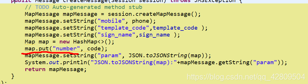
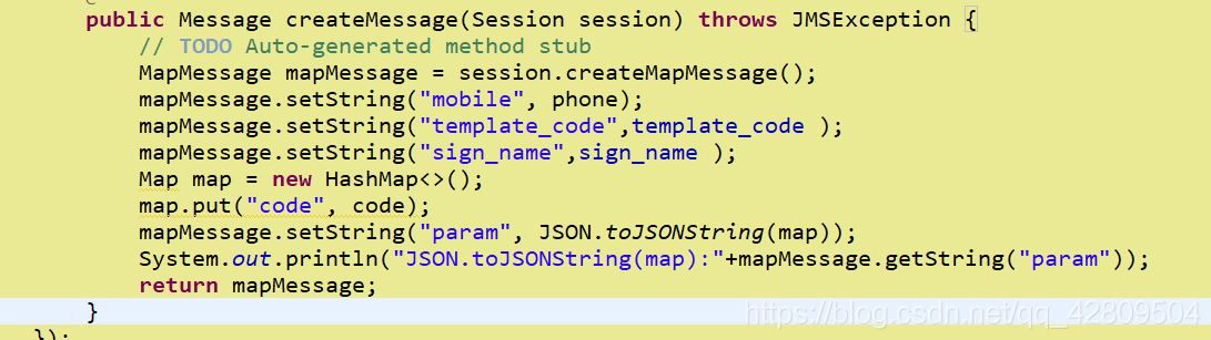
 解决阿里云短信服务参数错误
 本文介绍了一种常见问题,即使用阿里云短信服务时因参数名与模板要求不符而导致的错误。具体表现为模板需要的变量为'code',但实际提供的参数名为'number'。文章提供了简单有效的解决方案:将参数名更正为模板所要求的'code'。
 1073
1073

 被折叠的 条评论
为什么被折叠?
被折叠的 条评论
为什么被折叠?
 到【灌水乐园】发言


