《论文阅读》Linformer: Self-Attention with Linear Complexity

留个笔记自用

Linformer: Self-Attention with Linear Complexity

做什么

点云的概念:点云是在同一空间参考系下表达目标空间分布和目标表面特性的海量点集合,在获取物体表面每个采样点的空间坐标后,得到的是点的集合,称之为“点云”(Point Cloud)。
点包含了丰富的信息,包括三维坐标X,Y,Z、颜色、分类值、强度值、时间等等,不一一列举。在这里插入图片描述
一般的3D点云都是使用深度传感器扫描得到的,可以简单理解为相比2维点,点云是3D的采样
在这里插入图片描述

做了什么

这里设计了一款transformer变种,证明了自我注意机制也就是self-attention可以用一个低秩矩阵来近似,于是可以将时间复杂度O(n2)缩减至O(n)的线性transformer

怎么做

回忆一下常见的SA计算方法
在这里插入图片描述
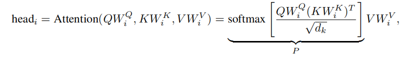
这里的三个W均是学习的矩阵,QKV就是常见transformer中的查询向量、键向量、值向量,对比之前论文里出现的
在这里插入图片描述
在这里插入图片描述
这里把括号里的softmax等部分称为P(上下文映射矩阵)∈Rn×n,就是点与点之间的attention矩阵,然而计算这个P非常昂贵,需要O(n2)的时间复杂度
然后画了两张图来进行分析
在这里插入图片描述
上面是两张频谱分析图,Y轴是上下文映射矩阵P的归一化累积奇异值,X 轴是最大特征值的索引,也就是将奇异值分解应用到模型的不同层和不同头部的P中,从上面这张图可以看的出,128之前整体曲线效果已经基本饱和,这意味着矩阵P的大部分信息可以从最初几个最大的奇异值中恢复出来
在这里插入图片描述
然后是一张不同层和头部的第128个最大特征值的归一化累积特征值的热图,观察到在较高层中,更多的信息集中在最大奇异值中,并且秩较低
简单来说,这里就是绘制了两张图,为了证明一点,高维度数据对处理这个任务来说起到的帮助较小,可以尝试将复杂度降低
为了使SA归为线性时间复杂度,这里说是先是要证明P矩阵是低秩的
提出了一个定理
在这里插入图片描述
简单来说就是对于任意的QKV和三个的W矩阵,对任意VW(也就是V)的任意列,都存在一个低秩矩阵P使得
在这里插入图片描述
然后开始具体的证明
重新换一个方式定义一下P
在这里插入图片描述
softmax的数学计算是
在这里插入图片描述
这里就将P的softmax里面假设为矩阵A,形式就可以改写成exp(A),D是一个n×n的对角矩阵
这里证明文中说是用了一个什么distributional Johnson–Lindenstrauss lemma
于是去查了一下这个的意思:严格说来是这样:在 M 维空间中的 N 个点,几乎总是被包含在一个 D 维子空间里的。这里的 D 按照直觉应当等于 N 的阶,可是实际上我们只需要让 D 是 log(N) 的阶就可以了。这里「几乎被包含在」的确切含义是它在这个子空间上的投影几乎是等距的(允许有一个 ε 的误差,而常数 D/log(N) 就依赖于 ε)。很显然,这件事情在高维数据降维时有极重要的意义。
然后构造一个近似低秩矩阵
在这里插入图片描述
前面的exp(A)·DA就是前面定义的P,这里的R是一个k×n的矩阵,是一个独立同分布的正态分布(0,1/k),然后就可以利用上面的定理证明对于V的任意列w
在这里插入图片描述
存在
在这里插入图片描述
附录给出了具体的数学证明,太数学了,看看就好
在这里插入图片描述
在这里插入图片描述
总的来说,还是理解一下JL lemma的道理,这个定理的意思就是在一个高维的欧式空间(距离用欧式距离表示),我们想要把这些点移动到一个低维的空间, 当时要保证空间转换后,每两个点之间的距离几乎不变。就是把一个高维计算能降至低维,大大降低了计算难度
得到了P矩阵的低秩属性后,使用奇异值分解来得到近似
在这里插入图片描述
σi、ui和vi是第i大的奇异值及其对应的奇异向量
所以总的来说,这里就是可以利用Plow这个低秩矩阵来近似我们之前使用的P,来近似我们之前使用的A,来简化attention的计算,而得到低秩矩阵的方法,就是对P使用奇异值分解
然后就是具体模型结构的设计
在这里插入图片描述
在这里插入图片描述
相较于最普通的head计算
在这里插入图片描述
主要是多在了两点,第一,映射矩阵P的区别,这里构造了一个相似矩阵P∈Rn×k(原来的映射矩阵P是n×n的),具体方法则是加了一个E层也就是线性投影层linear projection matrices。第二则是在外部V加了一个F层,同样也是线性投影层(使其从从n×d投影到了k×d)
这两步很明显最大的变化就是从n维到k的转换,从o(n2)到o(n×k),然后再根据前面的JL lemma定理可以得到,如果k特别小也就是远小于n,近似等同于时间复杂度为o(n)
接下来就是这种方法的理论和证明
在这里插入图片描述
在这里插入图片描述
这里又应用了上面的JL lemma,总的来说就是证明了前面能这么假设的可行性和误差性

总结

1.通篇数学实在太恐怖,总的来说就理解了做法,就是加了两层projection层,然后它就变成线性复杂度了!改天再看看代码然后再回来补一下。
在这里插入图片描述

### Linear Complexity Self-Attention Implementation and Optimization Self-attention mechanisms have been pivotal in advancing the capabilities of deep learning models, especially within natural language processing tasks. Traditional self-attention has a quadratic time complexity relative to input length due to its computation involving all pairs of positions in an input sequence[^1]. However, linear complexity self-attention aims at reducing this computational burden. #### Efficient Implementations One approach towards achieving linear complexity involves approximating or restructuring how attentions scores are computed between tokens. For instance, instead of computing full pairwise interactions, one could use locality-sensitive hashing (LSH), which groups similar items into buckets without explicitly comparing every item against each other. This method significantly reduces the number of required comparisons while maintaining performance quality[^3]. Another technique utilizes random projections where high-dimensional vectors representing token embeddings get projected onto lower dimensions through structured matrices like Fastfood transforms. Such transformations preserve distances well enough so that subsequent operations remain effective yet require fewer resources than standard methods do[^4]. ```python import torch from performer_pytorch import PerformerLM model = PerformerLM( num_tokens=20000, dim=512, depth=6, heads=8, causal=True, feature_redraw_interval=1000, generalized_attention=True, kernel_fn='relu' ) text = "The quick brown fox jumps over the lazy dog" tokens = tokenizer.encode(text).ids # assuming you've defined `tokenizer` elsewhere input_tensor = torch.tensor([tokens]) output = model(input_tensor) print(output.shape) # should output something like torch.Size([1, seq_len, vocab_size]) ``` This code snippet demonstrates implementing efficient self-attention via the Performer architecture from PyTorch library, leveraging fast Fourier transform-based kernels for reduced complexity computations during training phases. #### Optimizations Techniques Optimizing these implementations often revolves around exploiting hardware acceleration features such as GPU tensor cores optimized specifically for matrix multiplications involved in attention calculations. Additionally, mixed precision arithmetic can further enhance speed by performing some parts of forward/backward passes using half-precision floating-point numbers when possible without sacrificing much accuracy. Memory efficiency gains come not only from algorithmic improvements but also architectural choices like chunked processing schemes dividing long sequences into smaller manageable chunks processed independently before being recombined later on. These strategies help mitigate memory overhead associated with large-scale transformer architectures operating under constrained environments[^2]. --related questions-- 1. How does Locality-Sensitive Hashing contribute to making self-attention computationally feasible? 2. What role do random projections play in optimizing self-attention algorithms? 3. Can you explain how specific hardware optimizations impact the performance of linear-complexity self-attention models? 4. In what ways might chunked processing improve both runtime and resource utilization compared to traditional approaches?
评论 1
添加红包

请填写红包祝福语或标题

红包个数最小为10个

红包金额最低5元

当前余额3.43前往充值 >
需支付:10.00
成就一亿技术人!
领取后你会自动成为博主和红包主的粉丝 规则
hope_wisdom
发出的红包
实付
使用余额支付
点击重新获取
扫码支付
钱包余额 0

抵扣说明:

1.余额是钱包充值的虚拟货币,按照1:1的比例进行支付金额的抵扣。
2.余额无法直接购买下载,可以购买VIP、付费专栏及课程。

余额充值