python底层的逻辑回归

python底层的逻辑算法：
回归：回归是统计学的一个重要概念，其本意是根据之前的数据预测一个准确的输出值。
逻辑回归是《机器学习》这门课的第三个算法，它是目前使用最为广泛的一种学习算法，用于解决分类问题。与线性回归算法一样，也是监督学习算法。
诸如：新闻分类、基因序列、市场划分等的一些根据特征划分的，用的都是逻辑回归。
输出的最终预测结果为：正向类（1）、负向类（0）。

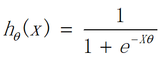
逻辑回归模型是一个“S”形的函数：

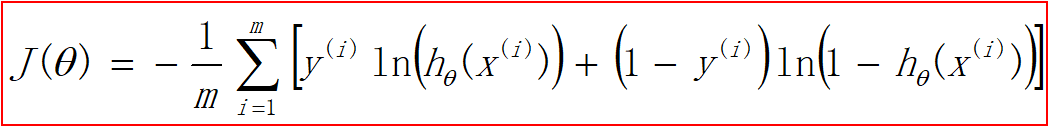
代价函数：代价函数 — 误差的平方和 — 非凸函数—局部最小点 。

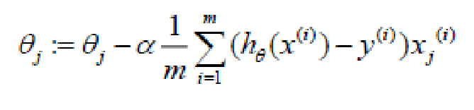
梯度下降

import numpy as np
import matplotlib.pyplot as plt
plt.rcParams['font.sans-serif']=['SimHei']
plt.rcParams['axes.unicode_minus']=False
train_data=np.loadtxt(r'LoR_linear.txt',delimiter=',')
test_data=np.loadtxt(r'LoR_nonlinear.txt',delimiter=',')

train_X,train_y=train_data[:,:-1],train_data[:,-1]
test_X,test_y=test_data[:,:-1],test_data[:,-1]

def preProess(X,y):
    #特征缩放
    X -=np.mean(X,axis=0)
    X /=np.std(X,axis=0,ddof=1)

    X=np.c_[np.ones(len(X)),X]
    y=np.c_[y]
    return X,y

train_X,train_y=preProess(train_X,train_y)
test_X,test_y=preProess(test_X,test_y)

def g(x):
    return 1/(1+np.exp(-x))
x=np.linspace(-10,10,500)
y=g(x)
plt.plot(x,y)
plt.show()
def model(X,theta):
    z=np.dot(X,theta)
    h=g(z)
    return h

def costFunc(h,y):
    m=len(y)
    J=-(1.0/m)*np.sum(y*np.log(h)+(1-y)*np.log(1-h))
    return J

def gradDesc(X,y,max_iter=15000,alpha=0.1):
    m,n=X.shape
    theta=np.zeros((n,1))
    J_history=np.zeros(max_iter)

    for i in range(max_iter):
        h=model(X,theta)
        J_history[i]=costFunc(h,y)
        deltaTheta = (1.0/m)*np.dot(X.T,h-y)
        theta -= deltaTheta*alpha

    return J_history,theta

def score(h,y):
    m=len(y)
    count=0
    for i in range(m):
        h[i]=np.where(h[i]>=0.5,1,0)
        if h[i]==y[i]:
            count+=1
    return count/m
#预测结果函数，结果不是0就是1
def predict(h):
    y_pre=[1 if i>=0.5 else 0 for i in h]
    return y_pre

print(train_X.shape,train_y.shape)
J_history,theta=gradDesc(train_X,train_y)
print(theta)
plt.title("代价函数")
plt.plot(J_history)
plt.show()

train_h=model(train_X,theta)
test_h=model(test_X,theta)
print(train_h,test_h)

def showDivide(X,theta,y,title):
    plt.title(title)
    plt.scatter(X[y[:,0]==0,1],X[y[:,0]==0,2],label="负样本")
    plt.scatter(X[y[:,0]==1,1],X[y[:,0]==1,2],label="正样本")
    min_x1,max_x1=np.min(X),np.max(X)
    min_x2,max_x2=-(theta[0]+theta[1]*min_x1)/theta[2],-(theta[0]+theta[1]*max_x1)/theta[2]
    plt.plot([min_x1,max_x1],[min_x2,max_x2])
    plt.legend()
    plt.show()

showDivide(train_X,theta,train_y,'训练集')
showDivide(test_X,theta,test_y,'测试集集')

train_y1=predict(train_h)
print('预测的结果是：',train_y1)